Generative recommenders encode each item as a short token ID, generate those tokens from the user history one by one, keep only the 50 highest-probability partial sequences at each step, and finally rank candidates by the same generation probability. Tail items have low probability and are often dropped in the first one or two steps: on Amazon Industrial & Scientific, MiniOneRec's 50 candidates cover only 11.94% of tail targets in the test set; when the authors inject 25 extra tail candidates per user—135 new tail targets in total—none of them enter the top 10 under generation-probability ranking. CAPE does not retrain the model; at inference it counts from the training data which items co-occurred with the user history under the same users, retrieves 25 extra tail candidates with that count, and adds the count into the ranking score. On LastFM, TIGER's top-10 hit rate on tail targets rises from 3.94% to 17.19%; across the paper's experiments, per-request latency rises only 11–16%.
1. Setting the scene
Generative recommendation has been hot in industry, led by models such as TIGER and OneRec. Unlike dual-tower retrieval, it builds no vector index. Each item is first encoded as a short ID—say three tokens—called a semantic ID (SID); items with similar content or representation share the same first few tokens. At serving time the model reads the user history, generates the first token, then the second and third, and a complete ID is one candidate item.
Users need more than one candidate, so generation uses beam search: at each step only the B highest-probability sequences so far are kept and the rest are dropped. This paper sets B to 50 and ends with 50 candidates. Ranking uses no second model; candidates are sorted by the probability of generating that item ID and the top 10 are shown. Recall and ranking share one score.
The paper focuses on tail items, defined as the bottom 80% by training-set frequency—called the long tail below. They make up more than half of test targets: 57.8% on Amazon Industrial & Scientific (I&S below), 51.1% on Amazon Office Products (Office), and 64.2% on LastFM.
2. Why the long tail is pruned at retrieval
Beam search compares probabilities of partially generated prefixes. The paper proves an intuitive fact with the chain rule: a prefix's probability equals the sum of probabilities of all items that start with it (Proposition 2.2).
is the first tokens of an ID, the user history, an item, and the probability of generating a nonexistent ID (zero when normalizing only over legal tokens).
So whether a prefix survives depends on the summed probability of all items under it, not on the best single item. Maximum-likelihood training already assigns low probability to tail items, so their prefixes often fail to stay in the top 50 at the first step.
Can one simply boost prefixes of tail items? The authors check and find that 99.97%, 96.21%, and 99.95% of tail items on I&S, Office, and LastFM share their first token with at least one head item. Boosting that prefix also boosts the head items under the same prefix.
Ranking cannot recover what was lost. As long as the top 10 are chosen from 50 candidates, the best possible tail hit rate is the share of tail targets that landed in the candidate set. Anything dropped at retrieval cannot be recovered by any later reranker (Proposition 2.1).
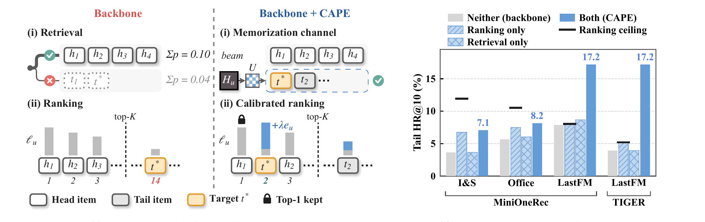
3. Diagnosis: where exactly is the long tail lost?
This experiment asks whether a tail target never enters the candidate set, or enters but is pushed down by ranking.
The trained model is held fixed. For each user three candidate sets are built and all are ranked by generation probability; the test target is checked for presence in the set and in the top 10. The three sets are: normal beam width 50; width raised to 75; width 50 plus 25 extra tail items—the 25 tail items with the highest co-occurrence with the user history that are not already in the original set. The co-occurrence algorithm is in Section 4.
Two models are used: MiniOneRec (generative recommendation on Qwen2.5-1.5B) on I&S, Office, and LastFM; TIGER (a classic encoder–decoder generative retriever) on LastFM, averaged over three random seeds.
| Data / model | Tail test users | Width 50: share of tail targets in candidates / top-10 hits | Width 75: share / top-10 | Extra 25: new tail targets in set / of which in top 10 |
|---|---|---|---|---|
| I&S / MiniOneRec | 2,622 | 11.94% / 96 | 14.45% / 95 | 135 / 0 |
| Office / MiniOneRec | 2,485 | 10.50% / 141 | 13.04% / 142 | 159 / 9 |
| LastFM / MiniOneRec | 634 | 8.04% / 50 | 9.31% / 55 | 98 / 6 |
| LastFM / TIGER | 634 | 5.21% / 25.0 | 5.63% / 25.0 | 107.3 / 0 |
Start with retrieval. At width 50 only 5.21%–11.94% of tail targets enter the candidate set; the remaining eight or nine tenths cannot be helped by any later ranking. Widening by 50% brings in 66 and 63 more tail targets on I&S and Office, but top-10 hits change by −1 and +1; on LastFM at most 8 more enter. The extra 25 beams still cover the next-highest-probability prefixes, which are mostly head items.
Then ranking. The extra 25 tail items do bring many targets in—135 on I&S—but after generation-probability ranking, 0 of them enter the top 10. Generation probability itself favors head items, so even when a tail target enters the set it ranks behind head items.
One more ratio will be used later: among tail targets missed at width 50, the share that rank in the user's top-50 tail items by co-occurrence with history is 8.2% on I&S, 9.6% on Office, and 24.0% / 25.5% on the two LastFM setups. Co-occurrence recovers clearly more on LastFM.
The authors attribute this to the memorization–generalization pair from Wide & Deep. Recommenders have two skills: remembering which two items co-occur (memorization) and generalizing to unseen combinations through shared representations. Generative models decide via shared prefixes and lean toward generalization; they lack item-pair memorization, which is exactly what item-based collaborative filtering provides.
4. Method: expand recall by one path, add one term to ranking
CAPE stands for Co-occurrence-Aware Pool Expansion. It changes no model parameters, no ID encoding, and no beam search; every change is added outside the model at inference. A request runs in three steps.
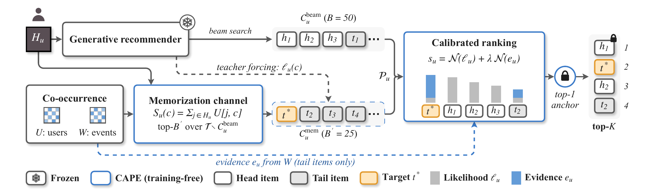
Step 1: add a tail-candidate path. Offline, build a table $U[j,c]$: how many users interacted with both item and item . Online, sum the rows of that table for each item in the user history to get , then take the top 25 among items that are tail and not already in the original 50. Counting users rather than interactions keeps a few heavy users from deciding what is added.
The 25 added items also need a model score to be ranked with the original set. Their IDs are fed to the backbone to compute the probability of generating each ID (teacher forcing in the paper)—one batched forward pass, with the user-history prefix shared. All 75 candidates then have a generation probability; co-occurrence only decides who enters the pool and does not replace the model score.
Step 2: add co-occurrence to the ranking score. Offline, build a second table $W[j,c]$: how often items and co-occur in the same training sequence; it keeps frequency of joint appearance that does not. A candidate's co-occurrence score is the average of its values with each history item, and is computed only for tail items—head items get 0. The final ranking score is:
is the log probability of generating item , is min-max normalization inside the 75 candidates so both scores sit in $[0,1]$, and is the only hyperparameter, controlling the weight of co-occurrence. Normalization is required because log probability and co-occurrence counts have different units and per-user distributions; after normalization the same works for every user.
Co-occurrence is limited to tail items because head items co-occur with almost everything, so the counts naturally favor the head. Adding the term to every candidate mainly boosts head items that already rank high.
Step 3: leave the first position alone. The first ranked item is always the backbone's first item; positions 2 through 10 are fully reranked by the new score. Every user still sees the same first recommendation as before, and HR@1 (the share of test targets hit at rank 1) stays unchanged.
is chosen on the validation set from {0, 0.05, 0.1, 0.25, 0.5, 1, 2, 5} by first requiring overall HR@10 (share of users whose top 10 hit the test target) to be no worse than the backbone, then picking the highest tail HR@10 among those values. All later baselines use the same selection rule.
Cost has two parts. Both tables are offline sparse CSR matrices: 1.8 MB and 2.4 MB per Amazon category, and 454 MB / 36 MB on LastFM's 40K songs. The main online cost is one forward pass to score the 25 added items; MiniOneRec already processes about 5,100 input tokens per request and adds about 100.
5. Experiments
Setup. Data are I&S and Office (MiniOneRec preprocessing: last 10 history items per user, 8:1:1 time split for train/val/test) and LastFM-1K (987 users, 40,429 songs). Every method uses beam width 50; baselines stay inside the same budget of 75 candidates and fall into two groups:
- Change retrieval: beam width 75; diverse beam search (DBS), which splits 75 beams into 5 groups with an inter-group diversity penalty.
- Change ranking on the same 75 candidates as CAPE: Frequency (subtract a popularity penalty from generation probability); MMR (trade off relevance and similarity to already chosen items); P-xQuAD (balance head and tail by the share of tail items in each user's history); NCP (add to every candidate—CAPE without the tail-only rule and without normalization). These four also lock the first position.
Main results ask two questions: can tail hit rate rise, and does overall hit rate fall. The table below is from the paper's Table 2, in percent.
| Data / model | Method | Overall HR@10 | Tail HR@10 | Tail NDCG@10 |
|---|---|---|---|---|
| I&S / MiniOneRec | Backbone | 12.57 | 3.66 | 1.62 |
| Width 75 | 12.57 | 3.62 | 1.61 | |
| Best reranker (P-xQuAD) | 12.88 | 4.58 | 2.12 | |
| CAPE | 12.46 | 7.06 | 3.42 | |
| Office / MiniOneRec | Backbone | 14.45 | 5.67 | 3.77 |
| Width 75 | 14.51 | 5.71 | 3.77 | |
| Best reranker (NCP) | 15.06 | 6.56 | 4.01 | |
| CAPE | 15.27 | 8.17 | 5.12 | |
| LastFM / MiniOneRec | Backbone | 7.50 | 7.89 | 4.62 |
| Width 75 | 8.11 | 8.68 | 4.89 | |
| Best reranker (NCP) | 9.73 | 11.20 | 5.50 | |
| CAPE | 12.06 | 17.19 | 8.18 | |
| LastFM / TIGER | Backbone | 5.10 | 3.94 | 3.02 |
| Width 75 | 5.10 | 3.94 | 3.02 | |
| Best reranker (NCP) | 9.46 | 9.88 | 5.46 | |
| CAPE | 12.33 | 17.19 | 8.49 |
Tail HR@10 rises 3.39, 2.49, 9.31, and 13.25 points over the backbone, and 2.48, 1.61, 5.99, and 7.31 points over the best same-candidate reranker. Overall HR@10 falls 0.11 only on I&S and rises 0.82, 4.56, and 7.23 on the other three.
The paper's explanations of why the baselines fail each have matching numbers. Frequency, MMR, and P-xQuAD stay within 1 point of the backbone's tail HR@10 on every dataset: popularity penalties and diversity only push tail items forward as a class and cannot tell which one the user wants. NCP also uses co-occurrence but adds it to every candidate, so head items are raised too, and it trails CAPE by 1.6–7.3 points. DBS after grouping produces many duplicate IDs—on I&S, 75 beams average only 28 distinct items.
On LastFM, after adding CAPE the two models' tail HR@10 become the same. Originally they differed by a factor of two—MiniOneRec 7.89 versus TIGER 3.94; with CAPE both are 17.19, with 109 and 108–110 hits (TIGER over three seeds), while overall metrics and HR@1 still differ. The authors' reading is that the two models lack the same kind of item-pair memorization on the tail; filling in the same co-occurrence information brings them to the same place, largely independent of model structure.
After freezing the method and the selection rule, the authors also run TIGER on three Amazon categories, including Beauty with more items (12,101). Tail HR@10 rises from 3.55 to 5.78, 3.43 to 5.75, and 1.34 to 2.12—relative gains of 58–68%—and overall HR@10 is never below the backbone.
How much do retrieval and ranking each contribute? Two ablations fix only one stage: retrieve-only keeps 75 candidates ranked by generation probability; rank-only does not expand the set and reranks the original 50 with the new score. Results are on the right of Figure 1.
Retrieve-only changes tail HR@10 by 0.00, 0.36, 0.79, and 0.00—added tail targets are pushed down by generation probability. Rank-only gains +3.05 and +1.81 on I&S and Office but stops exactly at 8.04 and 5.21 on LastFM, the share of tail targets already in the original set—the Section 2 upper bound. Doing both, the LastFM lift is far larger than the sum of the two parts: 9.31 versus 0.95 for MiniOneRec and 13.25 versus 1.26 for TIGER.
Which half matters depends on the data. On I&S and Office the backbone ranks only 31% and 54% of in-set tail targets into the top 10, so the bottleneck is ranking; rank-only raises those shares to 56% and 71%. On LastFM the backbone already ranks 98% (MiniOneRec) and 76% (TIGER) of in-set tail targets into the top 10, so ranking has little room and expansion is required; expansion alone beats rank-only by 9.15 and 11.99 points on LastFM versus 0.34 and 0.68 on Amazon. That matches the Section 3 ratios (Amazon 8–10%, LastFM 24–26%). Offline, those two ratios roughly tell whether gains will come from expanding recall or from changing the ranking score.
How to spend the extra 25 candidates. This compares beam width 50→75 with CAPE's co-occurrence expansion, both followed by the same new ranking score. The table is from the paper's Table 4; latency is wall-clock time for a full request on one GPU, mean over the first 128 test users per model, with relative multiples in parentheses.
| Data / model | Expansion | New tail targets in set | Tail HR@10 | Overall HR@10 | Latency (s) | Input tokens / request |
|---|---|---|---|---|---|---|
| I&S / MiniOneRec | Width 75 | 66 | 7.17 | 12.46 | 2.54 (2.41×) | 12,473 |
| Co-occurrence | 135 | 7.06 | 12.46 | 1.20 (1.14×) | 5,146 | |
| Office / MiniOneRec | Width 75 | 63 | 7.85 | 14.88 | 2.60 (2.42×) | 12,837 |
| Co-occurrence | 159 | 8.17 | 15.27 | 1.22 (1.14×) | 5,294 | |
| LastFM / MiniOneRec | Width 75 | 8 | 8.99 | 8.31 | 3.37 (2.41×) | 15,770 |
| Co-occurrence | 98 | 17.19 | 12.06 | 1.55 (1.11×) | 6,479 | |
| LastFM / TIGER | Width 75 | 2.7 | 5.47 | 5.98 | 0.35 (2.09×) | 545 |
| Co-occurrence | 107.3 | 17.19 | 12.33 | 0.19 (1.16×) | 291 |
On Amazon the two expansions are similar; on LastFM co-occurrence is more than 8 points higher. Cost differs a lot: widening the beam regenerates 25 extra sequences at every step, more than doubles input tokens, and adds 109–143% latency; co-occurrence expansion only scores 25 known IDs once and adds 11–16%.
The authors also replace co-occurrence expansion with a trained LightGCN retriever that likewise takes 25 items outside the original set, with ranking unchanged. LightGCN brings in only 14, 35, and 24 new tail targets versus 135, 159, and 98 for co-occurrence; across seven model–data combinations CAPE's tail HR@10 is always higher, by up to 9.3 points. Their explanation is that graph convolution smooths a tail item's signal onto its head neighbors, while raw co-occurrence keeps which two items actually appeared together.
The two most important ablations. The first checks whether added candidates help because they are co-occurring items, or only because 25 slots were reserved for the tail. Those 25 slots are filled with the 25 hottest tail items or with 25 random tail items. New tail targets fall to 9 and 26 on I&S, 33 and 21 on Office, and 0 on LastFM.
The second checks whether the ranking co-occurrence term helps because it remembers specific item pairs, or only because it uniformly boosts the tail. The item IDs in are randomly shuffled (mean of 5 runs) while the candidate set and the tail-only rule stay fixed. Tail HR@10 falls to 3.67, 6.04, 8.86, and 5.68—almost the same as ranking by generation probability alone. Together the two ablations show that the gains come from which items truly co-occurred with this user's history.
Two more groups. When co-occurrence is added to every candidate, not only the tail, overall HR@10 rises more (13.48, 15.82, 12.36, 13.41) while tail HR@10 trails CAPE by 0.24–2.71 points, and overall HR@10 beats the backbone on all four datasets. Generative models lack item-pair memorization overall, most on the tail; a business that cares more about overall metrics can drop the tail-only limit. Without locking the first position, HR@1 on the two Amazon categories falls from 5.58 to 5.47 and from 8.36 to 8.08—the lock costs little.
6. Limitations
Co-occurrence tables only cover item pairs seen in training; newly listed items with no co-occurrence records are unreachable on this path, and cold start is out of scope. The experimental scale is also small: Amazon keeps only 10 history items per user, LastFM has 987 users, and the largest model is 1.5B. How the two bottlenecks change with larger generative models or other ID encodings is, as the authors say, untested.
One more gap. LastFM's user-level co-occurrence table for 40K songs is already 454 MB; at industrial catalogs of tens of millions or more, a full item-pair table will not fit and must be truncated to each item's top-N co-occurring neighbors—cost and quality loss of that truncation must be measured separately.
7. What generative-retrieval teams can take away
The most portable piece is the diagnosis. Split test targets into head and tail by training frequency and count two ratios: how many tail targets land in the beam set, and how many of those in-set tail targets reach the top 10. That diagnosis needs no model change—only two ratios—and tells whether to expand recall or change the ranking score. If few in-set tail targets reach the top 10, change the ranking score first; if most of them already reach the top 10 but few enter the set, expand candidates outside the beam.
The method itself is also easy to land. It essentially plugs classic item-CF co-occurrence recall back into a generative pipeline: add one co-occurrence path outside the beam, score those items once with the generative model, and add a tail-only co-occurrence term to the ranking score. Many teams already run generative recall in parallel with traditional multi-path recall; this paper adds one conclusion: expanding candidates alone is not enough—added tail items are pushed down again by generation probability, so the ranking score must carry co-occurrence too. CAPE leaves the backbone's rank-1 item untouched and only rescores positions 2 through 10. That makes the launch blast radius easy to explain: the head result matches the backbone exactly, and only the later slots change.