 RecSys 2026
When a recommendation team maintains ranking models, contextual bandits, uplift models and sequential recommenders at the same time, it usually ends up with one library for matrix factorization, another for bandits, another for sequential models, and a separate set of glue code for evaluation, each with its own interface. To compare a ranking policy against a bandit policy on the same logs, the team has to make sure both sides are evaluated the same way by hand. Intuit's open-source scikit-rec puts all of this in one library: every recommendation pipeline is split into three layers, Recommender, Scorer and Estimator, and five recommendation paradigms share one evaluate(), which includes six off-policy evaluators plus an on-policy baseline. Its IPS, SNIPS, DR and DM estimates differ from the Open Bandit Pipeline (OBP) reference implementations by at most 4×10⁻¹⁶ relative. The companion scikit-rec-agent uses 15 structured tools to turn a plain-English description of data and goals into a trained, evaluated pipeline. An internal version has run at Intuit for 3+ years, powering 15 use cases across TurboTax and QuickBooks under a real-time latency requirement below 100 ms. The paper's contribution is a unified evaluation standard, not model accuracy, and the authors state explicitly that the experiments only serve to show the implementation is correct.
1. What existing libraries lack
The paper's Table 1 lists nine mainstream open-source frameworks. RecBole has 94 algorithms but only supports standard held-out evaluation; OBP only does off-policy evaluation for bandits and has no recommendation pipeline; Vowpal Wabbit supports contextual bandits and counterfactual evaluation, also without a recommendation pipeline; Merlin, TorchRec and TFRS focus on retrieval and ranking on GPUs. The authors conclude that no library puts ranking, bandits, uplift and sequential recommendation in one pipeline and compares them with one set of counterfactual evaluators.
Why not extend a framework like RecBole? The authors' reason is that those frameworks are organized around a fixed model catalog, so adding a new paradigm touches many places; in scikit-rec, a new paradigm is just one Recommender subclass.
2. The three layers
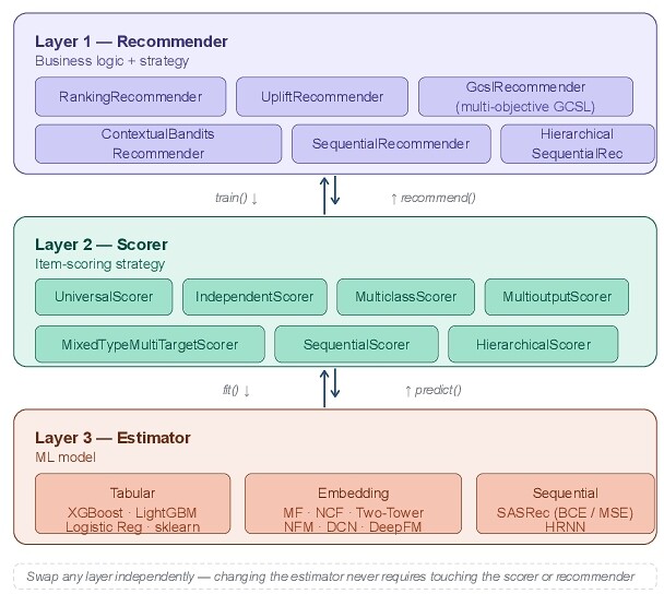
The Estimator is the underlying model, in three families. Tabular: XGBoost, LightGBM, sklearn models, and a pure-NumPy matrix factorization (ALS or SGD, no PyTorch needed). Embedding: MF, NCF, Two-Tower, NFM, DCN, DeepFM. Sequential: SASRec and HRNN (a hierarchical recurrent network with two GRU levels), both of which need PyTorch.
The Scorer decides how candidate items are scored for a user context. The most common is UniversalScorer: one global model whose input includes item features. IndependentScorer instead trains a separate model per item. There are also multiclass, multi-output, mixed-type multi-target, sequential and hierarchical scorers, seven in total.
The Recommender is the business-logic layer, one per paradigm: deterministic ranking (with optional temperature sampling), contextual bandits (epsilon-greedy and static-action exploration), uplift (treatment-effect estimation with T/S/X-Learners), SASRec-based sequential recommendation, and HRNN-based hierarchical sequential recommendation.
Once the contracts between layers are fixed, swapping XGBoost for a Two-Tower model is a one-line config change, with the Scorer and Recommender untouched. The data side is unified into three tables too, interactions, users and items, each declared by a YAML schema of required columns, dtypes and outcome fields, and validated at construction time.
3. One evaluate() over seven evaluators
This layer answers how policies from different paradigms can be compared fairly on the same logs. Logs are produced by the old online policy (the logging policy), and many items a new policy would recommend were never shown, so they have no real feedback. Off-policy evaluation (OPE) uses the old policy's logs to estimate how a new policy would perform online. The most basic estimator, IPS (inverse propensity scoring), is:
is the context of log entry , is the item shown at the time, is the feedback received, is the old policy's probability of choosing that item (the propensity), and is the new policy's probability of choosing it. Intuitively, the more a new policy favors items the old policy rarely chose, the larger the weight on those samples.
| Evaluator | Type | When to use |
|---|---|---|
| SimpleEvaluator | On-policy | Held-out test set, same policy |
| ReplayMatchEvaluator | Off-policy | Conservative; matched actions only |
| IPSEvaluator | Off-policy | Different policy; needs propensities |
| DREvaluator | Off-policy | Doubly robust; lower variance than IPS |
| SNIPSEvaluator | Off-policy | Self-normalized IPS |
| PolicyWeightedEvaluator | Off-policy | Weighted by new/old policy probability ratio |
| DirectMethodEvaluator | Off-policy | Reward model; no propensities needed |
The seven evaluators pair with twelve metrics (Precision, Recall, MAP, MRR, NDCG@k, ROC-AUC, Expected Reward and others). Recommendation scores are cached internally, so switching metrics or top-k cutoffs needs no new inference.
4. scikit-rec-agent: the LLM configures, it is not the model
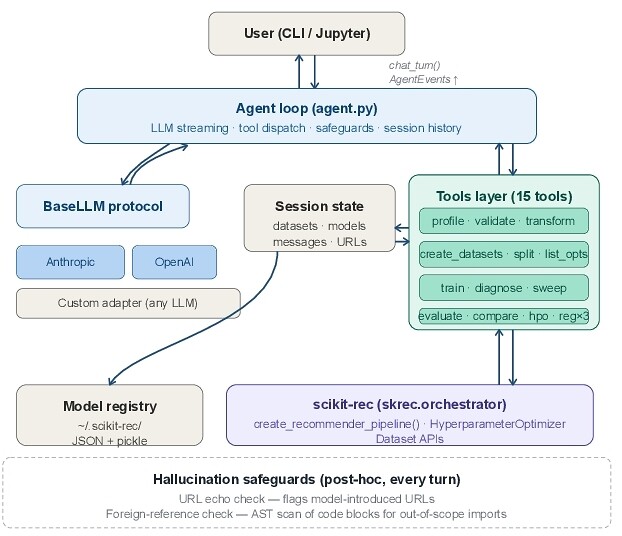
Choosing the Recommender, Scorer, Estimator, evaluator and data split takes a fair amount of domain knowledge. scikit-rec-agent wraps the whole workflow as a conversation: loading data, validating schemas, splitting, training, diagnosing failures, comparing many methods in a batch, tuning hyperparameters and saving models, 15 tools in all. A few design details:
- Datasets and models in session state are indexed by ID; only metadata enters the LLM context, never Python objects.
- "Which pipeline to recommend" is not a tool. The LLM gives 2–5 config dicts with rationales directly in its reply for the user to pick from, and config validity is checked by the pipeline factory, so the decision stays in the auditable conversation record.
- Two deterministic checks run on every output: a URL-echo check flags links the user never supplied and the system prompt does not contain; a foreign-reference check uses an AST scan of code blocks to flag imports outside the trusted set. Warnings are not written into conversation history, so the LLM cannot learn to evade them.
Every pipeline it produces is an ordinary scikit-rec composition, and the LLM takes no part in online scoring. In regulated settings where opaque model decisions are not allowed, this keeps every produced model auditable and reproducible. The preliminary evaluation is rough: on 5 internal Intuit datasets and 5 public ones, every pipeline the agent produced ran end to end, as checked separately by two authors by hand with full agreement; in an informal 20-prompt probe, the URL-echo check caught 5 non-existent links the LLM made up.
5. Design choices driven by production
Section 5 of the paper describes several design choices worked back from Intuit's production use cases:
- Scorer as its own layer. QuickBooks moved from "one propensity model per product" to a unified next-best-action recommender; the two setups differ only at the scoring layer, IndependentScorer versus UniversalScorer. The migration only swapped the Scorer argument, leaving the Recommender, Estimator and evaluation code untouched.
- recommend_online. The standard recommend() does a pandas merge across the interactions, users and items DataFrames, which is fine for batch scoring, but TurboTax's single-user real-time requests have a budget below 100 ms and the join overhead dominates. recommend_online skips the merge, takes pre-split single-row inputs, and goes through a NumPy-only scoring path.
- XGBoost latency. The default predict_proba builds a new DMatrix on every call, validates feature names, and copies the input into contiguous memory. XGBClassifierEstimator converts to NumPy once, uses Booster.inplace_predict() to avoid the copy, and turns off feature validation (features were already validated at the schema stage).
6. Experiments: proving correctness, not competing on accuracy
Accuracy on MovieLens-1M. The goal is to show each model's implementation lands in a reasonable range of published results. The protocol follows the NCF and SASRec papers: each user's last behavior is held out and ranked together with 100 random negatives, reporting HR@10 and NDCG@10.
| Model | HR@10 | NDCG@10 | Notes |
|---|---|---|---|
| BPR-MF (published) | 0.5781 | 0.3287 | Classical CF |
| Caser (published) | 0.7886 | 0.5538 | CNN sequential |
| SASRec original (published) | 0.8245 | 0.5905 | Reference impl. |
| MF-ALS (pure NumPy) | 0.7931 | 0.5421 | No PyTorch |
| SASRec (BCE) | 0.8953 | 0.6331 | Positives only |
| SASRec (MSE, ratings) | 0.8741 | 0.6102 | Soft labels |
| HRNN hierarchical sequential | 0.8612 | 0.5988 | Two-level GRU |
scikit-rec's SASRec scores higher than the original, and the authors say plainly that this comes from using only rating ≥4 behaviors as positives, a cleaner sequential signal, not from a method improvement, so the two are not directly comparable. The rows that can be compared directly are the scikit-rec ones, which share identical data preparation, splits and negative sampling.
OPE correctness. The goal is to show the off-policy evaluators have no numerical implementation errors. The data is ZOZOTOWN's Open Bandit Dataset with 80 actions; logs from a random policy are used to estimate the value of a Bernoulli Thompson Sampling policy, whose true value is 0.0042, with 20 bootstrap resamples. The IPS, SNIPS, DR and DM estimates differ from the OBP reference implementations by at most 4×10⁻¹⁶ relative.
| Estimator | Estimate | Bias | Rel. RMSE |
|---|---|---|---|
| IPS | 0.00417 | 2.6×10⁻⁵ | 0.231 |
| SNIPS | 0.00435 | 1.5×10⁻⁴ | 0.251 |
| DR | 0.00393 | 2.7×10⁻⁴ | 0.221 |
| Replay-Match | 0.00356 | 6.4×10⁻⁴ | 0.196 |
Only a 10K-row sample is used here, so the IPS family's relative RMSE sits around 25%; the authors say the full 26M-row release is needed for tight intervals. An OPE implementation bug raises no error; it just quietly picks the wrong policy, so matching the reference implementation bit for bit is more useful than reporting a nice-looking metric.
7. Limitations and what to try
Gaps the authors list: retrieval is still brute force, with no approximate-nearest-neighbor index such as FAISS or ScaNN; bandits have only epsilon-greedy and static-action, no Thompson Sampling or LinUCB; adversarial testing of the agent and a held-out task benchmark are not done yet, and the URL-echo check has known gaps. Also, the uplift paradigm is validated only on synthetic data and the TurboTax production use case; public rating data has no treatment assignment, so the paper has no accuracy numbers for it.
What to try:
- If your team runs ranking and bandit policies side by side, you can use its evaluate() to run IPS, DR and Replay-Match on the same logs and first confirm both sides are evaluated the same way.
- If your team implements its own OPE, you can follow the paper and check your numbers once against OBP bit for bit on the Open Bandit Dataset.