 RecSys 2026
Generative recommendation encodes each product as a few layers of discrete semantic IDs (SIDs), and the model generates these IDs layer by layer to perform retrieval and ranking. This Shopee paper points out one gap between it and discriminative ranking models: when a discriminative model scores a candidate it sees the product's category, shop and brand directly and crosses them with user features, while a generative model has seen no product-side information at all before it generates the first SID layer. UniRec's core technique is Chain-of-Attribute (CoA): the model first generates the product's category and then generates the SID conditioned on that category, which puts back into the decoding path the product features a discriminative model can use. Alongside it come an SID construction that caps codebook load by exposure, CDC that injects scenario and combination features into decoding, and business alignment via RFT plus DPO. Offline HR@50 is 22.6% higher (relative) than the strongest baseline OneRec-V2; launched on Shopee's main feed and landing pages, orders rose 4.76% and GMV 5.60%, with 110ms end-to-end latency versus 266ms for the original multi-stage pipeline.
The paper's arXiv title is "UniRec: Bridging the Expressive Gap between Generative and Discriminative Recommendation via Chain-of-Attribute"; this write-up is based on the arXiv full text.
1. Where generative recommendation falls short
A discriminative ranker estimates , the probability that user engages () given product features , with all product features visible at scoring time. A generative model generates the SID layer by layer as , and when generating the first layer it sees only the user, no product features.
The authors use Bayes' rule to show where the gap comes from:
does not vary across products, so ranking by the discriminative score is equivalent to ranking by , and the latter, expanded by the chain rule, is exactly generating product features one by one. The conclusion: if a generative model generated all of a product's features one by one, its ranking ability would equal the discriminative model's. Real systems cannot generate all features one by one because latency would be too high, so they compress product semantics into a few SID layers. Structured attributes such as category, shop and brand, which discriminative models cross directly, are folded into the SID during compression and no longer appear explicitly at decoding time, and that is where the gap comes from.
2. Method
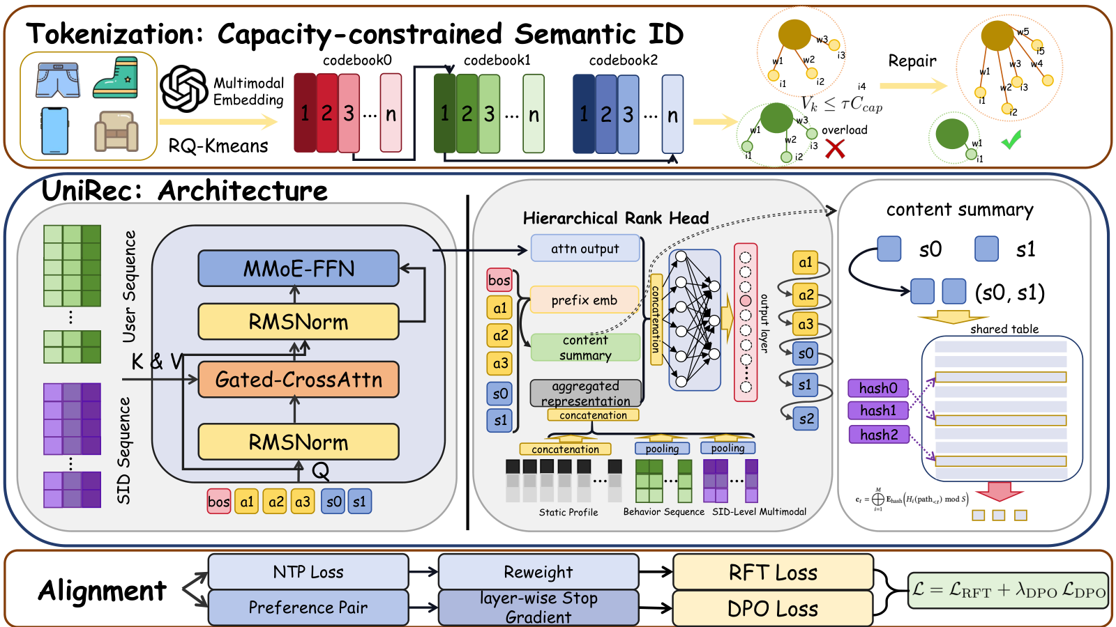
2.1 Chain-of-Attribute: generate the category first, then the SID
CoA prepends attribute tokens to the SID sequence, so generation goes attributes first, SID second:
In the production configuration the attributes are the product's second- and third-level categories (categories have three levels L1, L2, L3, getting finer going down), so a product's decoding path is "L2 category → L3 category → → → ", two steps longer than before.
Why generating the category first helps: products in the same category sit close together in SID space, so once the category is known, the candidate range for the next SID layer shrinks. The authors write this as the reduction in conditional entropy , which equals the conditional mutual information between the attributes and that SID layer and is greater than 0 whenever the two are correlated. With a lower error probability at each layer, the probability of getting the whole path right goes up, and beam search becomes more stable.
2.2 Capacity-constrained SID: balance the codebook by exposure, not product count
Existing balanced quantization (such as the RQ-KMeans used in OneRec) gives each codeword a similar number of products, but product popularity is long-tailed, and an even product count does not mean even exposure. The authors measured on Shopee production data: ranked by exposure, the top 10% of first-layer codewords take 33.24% of exposure; the top 10% of (,) combinations take 87.90%; the top 10% of three-layer combinations take 89.62%.
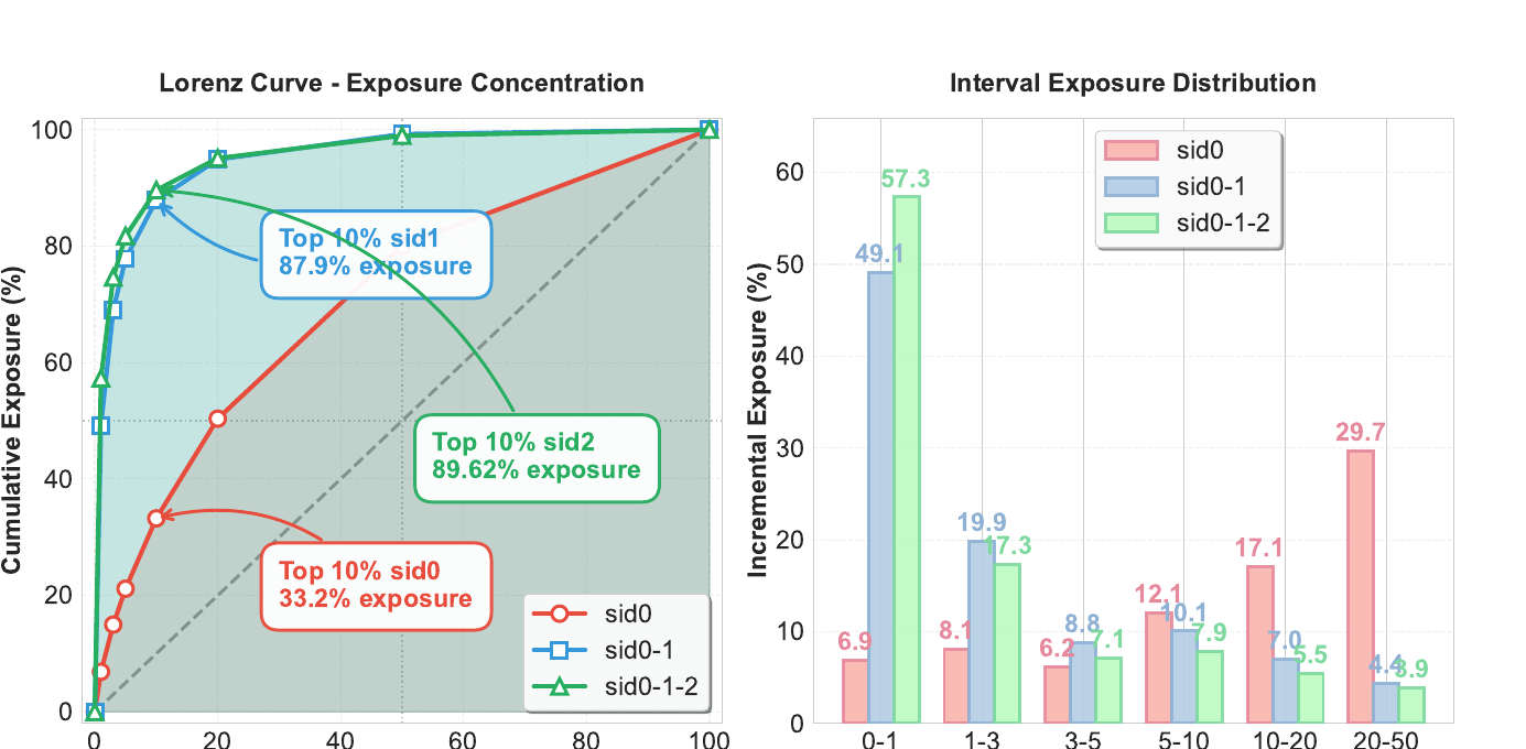
High-exposure token paths appear often in the training data, so the model keeps generating those few paths during beam search; the authors call this a Matthew effect inherited layer by layer. Capacity-constrained SID adds one constraint to the residual clustering at each layer: the sum of exposure weights of the products in each cluster may not exceed times the average load.
is product 's residual vector at the current layer, the cluster it is assigned to, a cluster center, its historical impression count, total exposure divided by the number of clusters, and in production. Solving this exactly is NP-hard, so a two-step greedy procedure is used: assign each product to its nearest cluster, then move products from overloaded clusters to the nearest cluster that is not full, repeating until reconstruction error stops changing.
2.3 CDC: tell the model which task it is on, then add combination features
One generative model has to serve objectives such as click, purchase, add-to-cart and cross-border, and scenarios such as main feed, search, similar items and flash sale. Task-Conditioned BOS replaces the fixed start token with a learnable vector looked up by "objective × scenario", steering decoding toward that scenario's distribution from the first step.
Content Summary deals with the combined meaning of tokens: the same following different categories may stand for completely different products. Giving every token pair its own embedding would mean about 16 million combinations for two layers with 4,000-token vocabularies. CDC instead uses 3 hash functions ($x+y$, , , with , primes) to map combinations such as (L2 category, ), (L3 category, ) and (, ) into one shared hash embedding table, concatenated into each step's combination feature .
2.4 Decoder and business alignment
The decoding-side sequence [BOS, attribute tokens, SID tokens] is Q; the item vectors of the user's latest 200 clicks, followed by 100 multimodal vectors fused from multi-layer SID embeddings, together form K and V, passing through 3 layers of cross-attention with a learnable gating coefficient and an MMoE-FFN. Each step has its own Rank Head, which concatenates the attention output, the embedding of the prefix generated so far, and the aggregated user representation, and outputs that step's token distribution through SENet and MaskNet.
Next-token prediction only fits the impression distribution and does not optimize GMV directly. RFT computes a business reward for each sample, subtracts the batch mean, divides by the root mean square and clips to get , and multiplies the sample's loss weight by . DPO builds preference pairs from items impressed under the same request, with purchase > click > impression only, and back-propagates only through the last SID layer while the predictions of earlier layers are left unchanged, so alignment does not disturb the prefix. The two are trained together:
In production the RFT to DPO loss weight ratio is 20:3, and DPO's .
3. Experiments
3.1 Main results
This experiment is meant to show that UniRec's retrieval quality is higher than existing generative and discriminative methods. The data is 9 consecutive days of Shopee main-feed production logs, billions of interactions. HR@K generates the top K candidates with beam search and checks whether the target product is among them; "order samples" counts only samples that ended in a purchase. Baselines: SASRec, a self-attention sequential recommender that does nearest-neighbor retrieval over the SID codebook with its learned representation; TIGER, generative retrieval with an encoder-decoder architecture; OneRec-V2, decoder-only generative retrieval with cross-attention. All three generative models have 0.05B parameters.
| Method | HR@50 | HR@100 | HR@200 | Order HR@50 | Order HR@100 | Order HR@200 |
|---|---|---|---|---|---|---|
| SASRec | 0.421 | 0.489 | 0.556 | 0.548 | 0.631 | 0.709 |
| TIGER (0.05B) | 0.437 | 0.508 | 0.578 | 0.567 | 0.652 | 0.731 |
| OneRec-V2 (0.05B) | 0.438 | 0.523 | 0.587 | 0.582 | 0.671 | 0.752 |
| UniRec (0.05B) | 0.537 | 0.618 | 0.688 | 0.672 | 0.774 | 0.867 |
On all samples UniRec is 9.5 to 10.1 points above OneRec-V2; on order samples it is 9.0 to 11.5 points higher. The authors attribute the gain on order samples to Task-Conditioned BOS separating click and purchase objectives and to RFT weighting samples by GMV.
3.2 Which attribute chain to use
This experiment answers which category level is best to put in front of the SID. It compares no attributes against different category combinations, looking at both each step's token Top-3 hit rate and the final HR.
| Attribute chain | @3 | @3 | @3 | HR@50 | HR@100 | HR@200 |
|---|---|---|---|---|---|---|
| No attributes | 0.314 | 0.752 | 0.952 | 0.458 | 0.532 | 0.595 |
| L1 → SID | 0.488 | 0.776 | 0.961 | 0.471 | 0.569 | 0.622 |
| L2 → SID | 0.591 | 0.789 | 0.963 | 0.515 | 0.597 | 0.664 |
| L3 → SID | 0.654 | 0.801 | 0.967 | 0.517 | 0.601 | 0.670 |
| L2 → L3 → SID | 0.682 | 0.821 | 0.971 | 0.537 | 0.618 | 0.688 |
Without attributes the first SID layer's Top-3 hit rate is only 0.314; with the L2 and L3 categories added it rises to 0.682. The improvement is concentrated in the first layer because the first SID layer originally had no product-side condition at all, so adding category information shrinks its choices the most. The finer the category, the higher the first-layer hit rate; generating L2 → L3 in sequence works best.
3.3 Component ablations
This experiment is meant to quantify the contribution of capacity-constrained SID, Task-Conditioned BOS and Content Summary; each time one component is removed and compared with the full model.
| Configuration | HR@50 | HR@100 | HR@200 |
|---|---|---|---|
| Full model | 0.537 | 0.618 | 0.688 |
| SID with RQ-KMeans | 0.481 | 0.558 | 0.627 |
| w/o Task-Cond. BOS | 0.493 | 0.570 | 0.638 |
| w/o Content Summary | 0.485 | 0.565 | 0.637 |
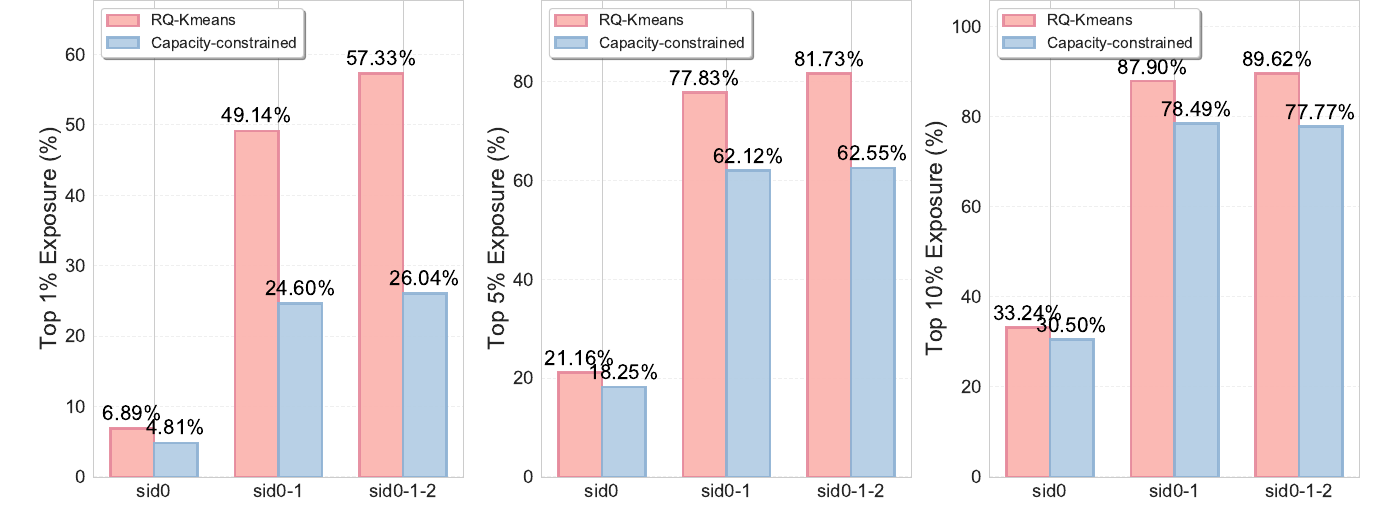
Removing any one of the three components drops HR@50 by 4 to 6 points. After switching back to RQ-KMeans, the authors also compared the exposure concentration of the two SIDs: on three-layer combinations, the top 1% of tokens take 57.33% of exposure under RQ-KMeans and 26.04% with the capacity constraint.
Task-Conditioned BOS also got a multi-scenario experiment: trained on mixed samples from three production scenarios, HR@100 is 0.470 with a separate model per scenario, 0.486 for mixed training without scenario prompts, and 0.510 with the scenario BOS. Mixed training helps by itself, and adding the scenario condition improves all three cutoffs a bit more.
Increasing model width from 64 to 512 raises HR@50 from 0.397 to 0.557, without saturating.
3.4 Online A/B
Online experiments ran on the main feed and landing pages, with the original discriminative multi-stage recommender as control and 20% of user traffic per bucket.
| Metric | Overall | Main feed | Landing page |
|---|---|---|---|
| Orders | +4.76% | +4.27% | +5.78% |
| GMV | +5.60% | +5.42% | +6.19% |
| Page-view CTR | +5.37% | +5.37% | — |
End-to-end latency is 110ms, comparable to a single ranking model; the original multi-stage pipeline took 266ms.
4. Limitations
The paper has no separate limitations discussion. Two points stand out from the experimental setup. First, all offline comparisons are on Shopee's internal data, with baselines also limited to 0.05B parameters, and there are no results on public datasets. Second, the online control is the entire discriminative multi-stage system, so the A/B gain includes the combined effect of the generative architecture, CoA, capacity-constrained SID, CDC and alignment; the paper gives no per-component online contribution.
5. Practical implications
- If the first-layer SID hit rate of your generative retrieval is low, try CoA first: put one or two category levels in front of the SID, at the cost of only two extra decoding steps; in Table 2 the first layer's Top-3 hit rate rose from 0.314 to 0.682.
- When building SIDs, check exposure concentration, not just whether product counts are even. A codebook balanced by product count can still let a few popular combinations take nearly 90% of exposure, and beam search will keep walking those few paths; adding an exposure-based capacity constraint only changes the clustering assignment step, so the cost is low.