SHARE

Since Ampere, NVIDIA GPUs have supported 2:4 sparsity: in a matrix multiplication, one operand keeps only two non-zeros in every four elements along the reduction axis, and the tensor cores nominally run twice as fast. It can be stacked with quantization, so the real deployment question is: from the current precision, should the next step be adding 2:4 or dropping to the next lower precision? This paper by an independent researcher compares the two on Llama-3.1-8B-Instruct and Qwen3-8B, at "equal storage bits (with the sparsity position index counted)" and at "equal nominal compute tier". It covers all six GEMM operand families of a transformer layer that could be sparse (linear-layer weights and inputs, and attention queries, keys, values and probabilities), and times them on three GPU generations (L40S, H100, RTX PRO 6000), over 220,000 configurations in all. The conclusion is blunt: as long as a lower precision is available, adding 2:4 is both less accurate and slower. Only at the lowest precision the hardware supports (FP8 on Ada and Hopper) does 2:4 earn its place: on an H100, a 2:4 plus FP8 model served by vLLM gets 27% higher prefill throughput than dense FP8 with GSM8K accuracy on par. But that model was retrained on 13 billion tokens; one-shot pruned models are unusable.
1. The problem: hardware still supports it, software has given up
On one side, NVIDIA has kept sparse tensor cores in every GPU generation, and Blackwell added sparse FP4; on the other, in 2026 vLLM and LLM Compressor removed 2:4 support because too few people used it. A split this wide shows that a direct comparison on real hardware is missing.
Existing pruning-versus-quantization comparisons mostly compare at "nominal compression", mostly for weights, and do not time "add 2:4" against "drop one precision" on the same GPU. The author points out four things that are easy to miss. First, 2:4 stores a position index next to every kept value, so it costs more than half the bits of its dense counterpart. Second, both approaches promise twice the throughput, but the datasheet does not say how much each actually delivers. Third, most operands at inference time (activations, Q, K, V, attention probabilities) are computed on the fly and must be pruned and compressed before every GEMM, a cost invisible if you time only the GEMM. Fourth, the hardware fixes which operand can be sparse and along which axis, so whole-tensor statistics (such as kurtosis) miss what 2:4 actually removes.
2. How to compare fairly
The first yardstick is equal bits, for comparing memory savings. Each format is charged for every bit it stores per original element: values, indices and scales. 2:4 keeps half of the elements but adds a 1-bit index per original element, so it saves less than half of the bits. The result is that "2:4 on 2m-bit values" costs exactly as much as "dense (m+1)-bit": 2:4 with INT8 costs the same as dense INT5, 2:4 with INT4 the same as INT3, and 2:4 with FP16 costs more than FP8.
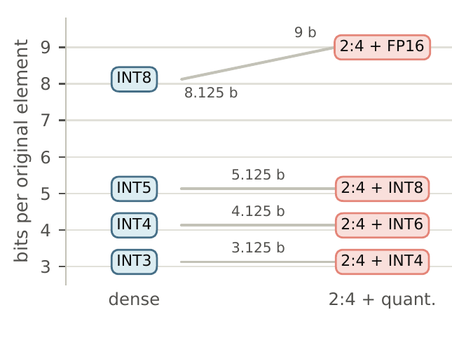
So at equal storage, the real choice is "drop half the elements and store each of the rest in bits" versus "keep all elements at bits each".
The second yardstick is equal compute tier, for comparing speedups: pair formats by datasheet nominal throughput. The 2x tier is 2:4 with FP16 against dense FP8 or INT8; the 4x tier is 2:4 with FP8 against dense 4-bit floating point, which only Blackwell has.
Under both yardsticks, accuracy is operator-level relative error against an FP32 reference output. The author defines R as "error of the best 2:4 configuration" divided by "error of the best quantized configuration"; R below 1 means 2:4 is better. To favour neither side, each picks the best from an equal-effort menu: the 2:4 side tries three pruners: magnitude pruning, which drops the smallest weights; Wanda, which ranks weights by magnitude times the activation size of their input; and SparseGPT, which after pruning adjusts the remaining weights with second-order information from calibration data. The quantized side also tries three: plain round-to-nearest; GPTQ, which quantizes column by column and pushes the error onto columns not yet quantized; and AWQ, which scales up the weights of channels with large activations before quantizing, to protect them. Both sides calibrate on the same C4 data. Speed uses cuSPARSELt sparse GEMMs, and for operands computed on the fly both sides pay for online pruning or online quantization.
3. While a lower precision exists: dropping one step always wins
On accuracy, at equal bits 2:4 loses at every storage budget on both models. At the most generous budget (the dense side in an 8-bit format, which by the conversion above lets the kept 2:4 values use about 14 bits), the error gap is over an order of magnitude; it shrinks as bits fall but never flips, and the closest case still has R just above 1. At equal tiers it is clearer: in the 2x tier, 2:4 with FP16 has five to sixteen times the error of dense FP8, for all six operand families. Across all compute comparisons, the few cases 2:4 wins are against weak formats: MXFP4 (4-bit floating point where every 32 elements share one scale restricted to a power of two, a coarse scale) and INT8 with a single scale per row. Against FP8 and NVFP4 (also 4-bit floating point, but with an FP8 scale per 16 elements plus one per tensor, a much finer scale) it never wins.
Operator error is not model quality, so the author also ran whole-model tests on the 15 configurations closest to parity, the most favourable cases for 2:4. On GSM8K, 2:4 is never significantly better than quantization and is significantly worse 7 times. RULER is a long-context benchmark that tests finding and using given information in long text. Where 2:4 is significantly better than its quantized rival on perplexity or RULER, it is mostly on attention probabilities: keeping the top two of every four scores sharpens attention, which helps long-context retrieval and perplexity but never helps reasoning.
Measured speed is just as unfavourable to 2:4. The table gives "rival time divided by 2:4 time"; above 1 means 2:4 is faster (Llama-3.1-8B projections, median over 2K to 16K tokens):
| GPU | 2x tier W | 2x tier X | 4x tier W | 4x tier X | 2:4 added on FP8 | 2:4 added on NVFP4 |
|---|---|---|---|---|---|---|
| L40S | 0.89 | 0.89 | – | – | 1.65 | – |
| H100 | 0.74 | 0.80 | – | – | 1.42 | – |
| RTX PRO 6000 | 0.84 | 0.85 | 0.66 | 0.70 | 1.33 | 1.40 |
W means the weights are sparse; X means the activations are sparse (online preprocessing counted on both sides). The first four columns are all below 1, which means that of two approaches promising the same nominal speed, dense lower precision delivers more in practice. On H100, 2:4 with FP16 runs at only 74% of dense FP8's speed.
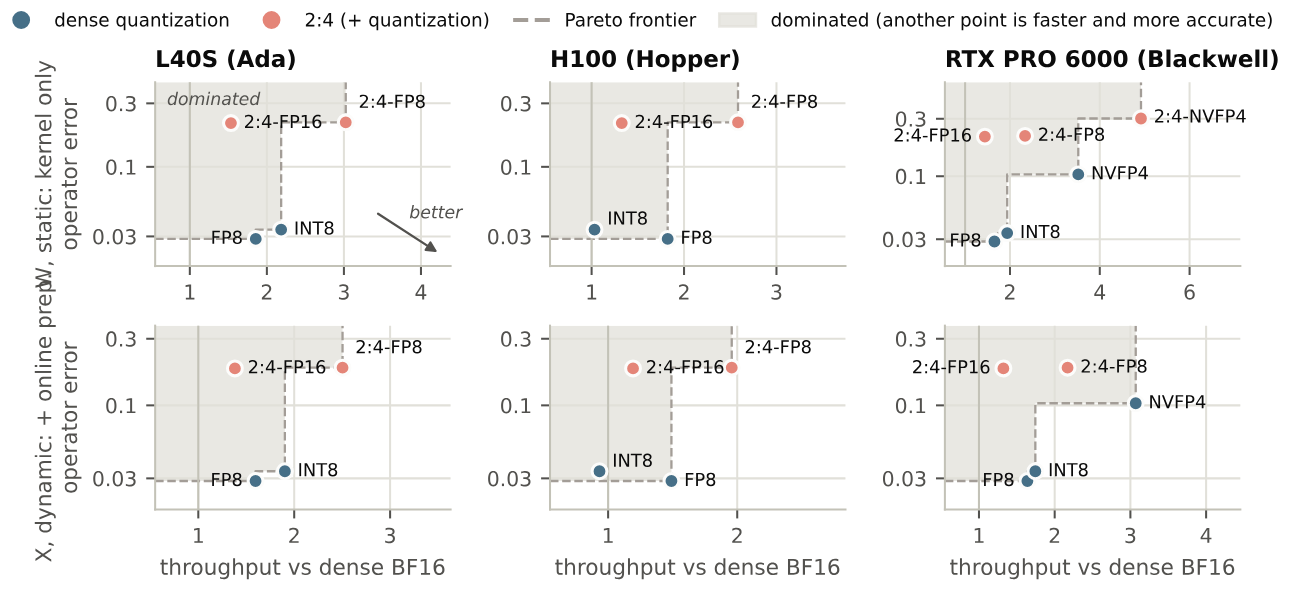
Putting accuracy and speed together, as long as a lower dense precision is available, every 2:4 configuration falls in the grey region: some dense format is faster and several times more accurate. 2:4 reaches the frontier only at the far right, once stacked on top of the lowest precision.
How online pruning is implemented also matters. The author wrote a fused kernel that reads the input once and writes kept values and indices once, running near memory-copy bandwidth; cuSPARSELt's own prune-and-compress path and PyTorch's semi-structured conversion are several times slower and eat most of what the sparse GEMM saves. Attention probabilities P are even worse: after online pruning and compression, 2:4 runs at about half the dense speed, so P cannot be used as a standalone sparse operand.
4. Why it loses: the deleted energy cannot be won back
The reason is a simple asymmetry. Quantization keeps every value and only rounds it; each added bit halves the error. 2:4 deletes half the values outright; what is deleted is gone, and no number of bits on the remaining values brings it back. The author adds up the squares of the dropped values over all groups of four and divides by the sum of squares of the whole tensor, calling this the "2:4 energy loss". For i.i.d. Gaussian data it is 13.2%, independent of bits. On Gaussian data the 2:4 side's error stays at 36% to 37% across budgets, while the dense format of equal bits goes from 0.6% at INT8 to 27.4% at INT3. The two would cross only below 3 bits, a precision no dense tensor core supports.
Once the mask is fixed, dropped values carry only pruning error and kept values only quantization error. They sit on different elements, so their squared errors (error energies) add exactly; every error below means relative error energy, divided by the tensor's total sum of squares, and its square root is the relative error, so a 13.2% energy loss is about 36% relative error. The 2:4 side's error is "energy loss plus the error of quantizing the kept values to bits", the dense side's is "the error of quantizing all values to bits", and the square root of their ratio is the predicted R. Every term is computed directly from the tensor, with no fitted parameters. Its rank correlation with measured R is 0.93, and it separates 2:4 wins from losses with an AUC of 0.95. But 2:4 wins at only 3% of points, so the criterion explains how big the gap is and why, not who wins a close call. For contrast, the whole-tensor kurtosis proposed in earlier work barely correlates with the outcome. What decides the contest is the local structure of the tensor along the hardware's grouping axis, not its overall distribution.
The analysis also predicts the effect of Hadamard rotation. Before low-bit quantization, tensors are often multiplied by a Hadamard matrix (an orthogonal matrix of ±1 entries, rescaled), which mixes each value with many others and spreads a few large outliers across many elements. Because of this spreading, the four elements in each group become more alike, so pruning two of them loses more energy; meanwhile the flattened outliers narrow the quantization range, so quantization error shrinks. Both effects work against 2:4. In measurements, rotation roughly doubles R for Q, K and linear-layer inputs, and the criterion predicts the direction of change at 87% of points. Most real deployments rotate, so the paper's unrotated results are actually optimistic for 2:4.
5. At the lowest precision: a real speedup, but only with retraining
At the FP8 or NVFP4 floor there is no lower dense format to switch to, so 2:4 can only be stacked on top, and at this point it has no rival. The author makes the linear-layer weights 2:4, keeps attention in BF16, and uses the base Llama-3.1-8B. Linear-layer GEMMs with 2:4 on FP8 run 1.3x to 1.7x faster, the first time in the paper that 2:4 really wins.
End-to-end vLLM results on one H100; the 2:4 model is Sparse-Llama (a 2:4 Llama retrained on 13 billion tokens):
| Configuration | Weight memory (GiB) | Prefill (k tok/s) | Decode b=1 (tok/s) | Decode b=64 (tok/s) | GSM8K |
|---|---|---|---|---|---|
| Dense BF16 | 15.0 | 41.4 | 136 | 6,424 | 0.596 |
| 2:4 BF16 | 9.3 | 40.7 | 115 | 6,477 | 0.624 |
| Dense FP8 | 8.5 | 58.9 | 198 | 8,556 | 0.568 |
| 2:4 FP8 | 6.1 | 74.6 | 234 | 9,914 | 0.612 |
2:4 plus FP8 has 27% faster prefill than dense FP8, 18% and 16% faster decode at batch 1 and 64, and 28% less weight memory. The end-to-end gain is smaller than the GEMM-level 1.42x because attention and the other layers do not shrink. Serving the same weights with dense kernels removes the speedup, so the gain comes entirely from the sparse kernels. In BF16, vLLM's 2:4 path is no faster than dense, and slower at batch 1.
The GSM8K column needs care. With only 250 problems, at around 0.6 accuracy the standard error is about 3 points, so the gap between 0.568 and 0.612 is within noise, and the author also reports no significant difference. And the 2:4 model and the dense model have different training histories, so all one can say is "no worse", not "2:4 is more accurate".
The real cost is retraining. The table gives WikiText-2 perplexity and GSM8K accuracy (250 problems):
| Floor | Dense | One-shot 2:4 | Retrained 2:4 (13B tokens) | Author's retraining (1B tokens) |
|---|---|---|---|---|
| BF16 | 6.31 / 0.600 | – | 8.13 / 0.612 | 8.19 / 0.300 |
| INT4 weights | 6.90 / 0.540 | 18.61 / 0.032 | 8.45 / 0.580 | 8.53 / 0.292 |
| FP8 | 6.36 / 0.552 | 17.82 / 0.028 | 8.19 / 0.632 | 8.25 / 0.308 |
One-shot pruning is unusable on every floor: perplexity more than doubles and GSM8K drops to about 3%, which means the model has essentially lost its reasoning. The author's own distillation retraining from the dense model on 1 billion FineWeb-Edu tokens catches up with Sparse-Llama on perplexity (8.25 vs. 8.19) but gets only half its GSM8K (0.308 vs. 0.632).
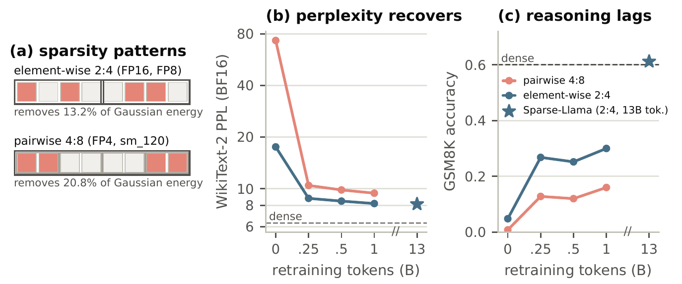
Perplexity overstates how much retraining has recovered: perplexity is mostly back within the first 0.25 billion tokens while reasoning is far from back, and the perplexity curve gives no hint of how far there is to go. Judging whether a sparse model's retraining is done requires a reasoning task. Sparsifying only some layers does not avoid retraining either: picking linear layers one by one from the lowest predicted error upward until they make up half the linear-layer compute, and applying 2:4 to them, buys only 1.14x to 1.25x.
6. Blackwell's sparse FP4 is harder to use
Blackwell's sparse FP4 is not element-wise 2:4 but "pairwise 4:8": each group of eight elements is split into four adjacent pairs, and two of the pairs are kept. The author verified on an RTX PRO 6000 that element-wise masks give wrong results in this format. Its kernels run 1.4x faster than dense NVFP4, but keeping pairs discards more than keeping elements, because both elements of a pair must stay or go together and cannot each be chosen by size. On Gaussian data its energy loss is 20.8%, and after one-shot pruning perplexity reaches 108.83, five times that of element-wise 2:4.
Existing models do not help either. Sparse-Llama, trained for element-wise 2:4, cannot be converted directly; conversion discards a third of its trained weights and breaks the model. With the author's 1-billion-token retraining budget, GSM8K recovers only to 0.132, against 0.460 for dense NVFP4, so at this budget it is not usable.
7. Limits and practical takeaways
- Only two 8B models. The Blackwell conclusion is limited by 1 billion tokens and one untuned retraining recipe; whether longer retraining recovers it is not tested.
- The 4-bit integer weight floor (mainly for decode) is not timed, because vLLM removed the matching sparse kernels. Decode is bound by memory bandwidth, where 2:4 saves only bytes, which helps on some GPUs and hurts on others.
- In the speed comparisons, sparse GEMMs get an exhaustive tuning search while the dense side uses the library's default heuristics, which favours 2:4, and 2:4 still loses.
If the hardware still offers a lower precision (e.g. BF16 to FP8 on H100), drop the precision first; do not add 2:4. If you already deploy in FP8, prefill throughput is the bottleneck, and a well-retrained 2:4 model is available, 2:4 can give a real 20–30% speedup, but vLLM mainline has removed support, so you will be maintaining your own branch. On Blackwell, there is no ready pairwise 4:8 model yet, and the cost and outcome of retraining your own are not assured. When evaluating any retrained sparse model, do not rely on perplexity alone.
How did this read for you?
Hoot made a note. Thanks for the feedback.

One tap, no sign-in; tap again to undo. Only anonymous counts are kept, never who you are.
Discussion
Add experiment details, reproduction notes or a different take. Requires a GitHub sign-in.
Loading the discussion…