Contents · 8 sections
1What problem does it solve?2Where do existing metrics fall short?3PCE: calibration by quantiles4SPREE: adding a "popularity direction" inside the model5What do the experiments show?6Limitations as I see them7How a recommendation team could try it8Conclusion and assessmentSHARE

This paper is worth reading for teams that care about popularity bias in recommendation but do not want to retrain their models. The authors, from Amazon Music and the University of Amsterdam, look at popularity bias from a different angle. The problem is not that recommendations are too popular overall. The problem is that their popularity does not match each user's own taste. The paper does two things. First, it proposes PCE (Popularity Calibration Error), which compares, quantile by quantile, the popularity distribution of items in a user's history with that of the recommendation list. Second, it proposes SPREE (Steering PopulaRity toward human prEferEnces). At inference time, SPREE adds a "popularity direction" vector to the internal representation of SASRec. The sign and strength of that vector depend on each user's estimated bias, and no retraining is needed. On 4 public datasets, taking the strongest setting that loses at most 10% of NDCG@100, SPREE lowers PCE@100 by 4% to 16%. Applying the same direction uniformly to every user instead doubles PCE on two datasets (Table 4). I think the useful ideas are the goal of alignment rather than blanket de-popularization, and the quantile-based measurement. However, the experiments only use a small 64-dimensional, 3-layer model on public datasets, and the bias estimator reaches an R² of only 0.18 on the smallest dataset.
What problem does it solve?
Recommender systems commonly favor popular items, and this has been discussed many times. A common fix is to push popularity down across the board, for example by discounting scores by popularity. The paper argues that this can work against user experience. Some users simply love chart hits, while others only listen to niche bands. Uniformly lowering popularity annoys the first group and may still not be enough for the second.
So the authors reframe the problem as alignment. The items a user has interacted with form one popularity distribution, . The items the model recommends to that user form another, . An item's popularity is simply the total number of interactions it has across all user histories. An ideal recommender should make close to .
A schematic example: half of user A's history is popular songs and half is obscure songs, so the popularity distribution has two peaks. The recommendation list contains only moderately popular songs. The average popularity of the two may be similar, yet the recommendations completely miss the taste for both extremes.
Where do existing metrics fall short?
The paper uses measurement theory to sort existing popularity bias metrics by what they actually measure. One group measures how popular the system's recommendations are overall, such as ARP, the average popularity of recommended items. Another measures how concentrated exposure is across items, such as coverage or the Gini coefficient. The third measures how far each user's recommendations are from that user's history. This paper only cares about the third group and sets five requirements for it:
| Requirement | Meaning | PopLift | LogPopDiff | UPD | PCE | Calibration curve |
|---|---|---|---|---|---|---|
| D1 Direction | Tells whether recommendations are more or less popular than the history | ✓ | ✓ | × | × | ✓ |
| D2 Magnitude | Captures small differences too | ✓ | ✓ | × | ✓ | ✓ |
| D3 Dispersion | Tells whether recommendations are more concentrated than the history | × | × | × | ✓ | ✓ |
| D4 Scale invariance | Does not change with the number of users or interactions | ✓ | × | ✓ | ✓ | ✓ |
| D5 Outlier robustness | One extremely popular item does not skew the result | × | × | ✓ | ✓ | ✓ |
PopLift subtracts the mean popularity of the user's history from the mean popularity of the recommendation list and divides by the history mean, giving a relative difference. LogPopDiff takes the log of each item's popularity, averages each side, and subtracts the two directly without normalizing. Both look only at means, so they miss dispersion. LogPopDiff uses an absolute difference, so its value moves as total interactions grow, which breaks scale invariance. PopLift averages raw popularity, so a single very popular item can pull the mean up; the log in LogPopDiff softens this but does not remove it. UPD (user popularity deviation) cuts popularity into low, medium and high bins and then computes the Jensen-Shannon divergence between the two distributions. It cannot see differences within a bin. The divergence is also symmetric, so over-popular and over-niche recommendations get the same score.
PCE: calibration by quantiles
PCE borrows the idea of quantile calibration from regression models. For each user:
- Pick quantile levels , for example 0, 0.2, 0.4, 0.6, 0.8 and 1.
- In this user's recommendation list, find the popularity threshold at quantile . A fraction of the recommended items have popularity at or below it.
- Count the fraction of items in the user's history with popularity at or below that threshold, and call it .
- Ideally . PCE is the mean of the values of . It ranges from 0 to 1 and is then averaged over all users.
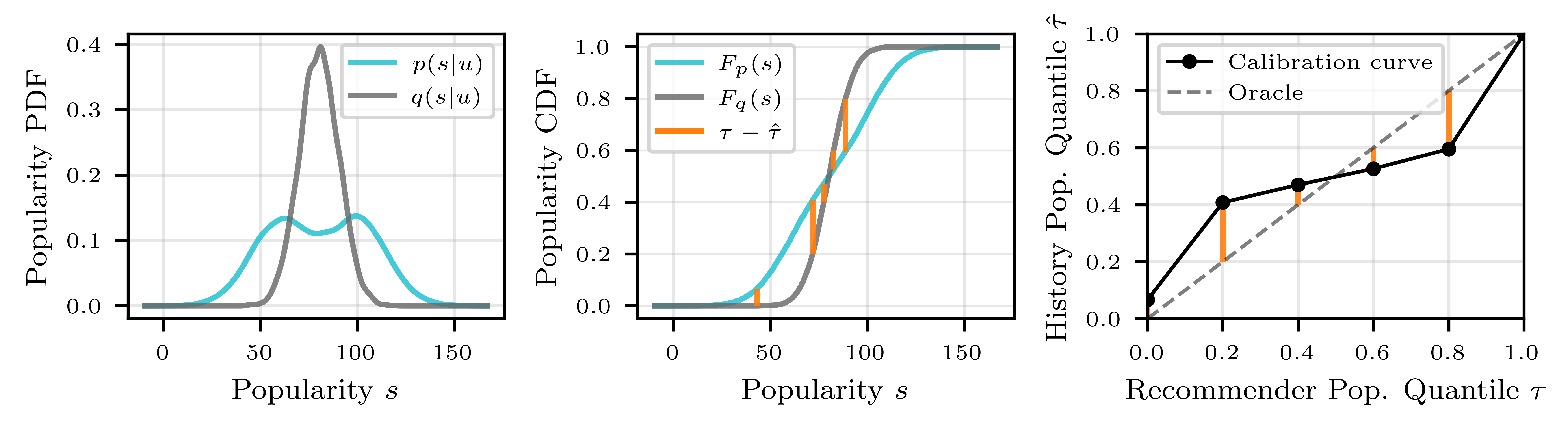
Let us work through user A by hand. All recommendations are moderately popular, so the 20% quantile threshold of the recommendations is already a moderate popularity level. Half of the user's history consists of obscure songs, all below this threshold, so , which is higher than 0.2. At the 80% quantile, the threshold is still moderate popularity, and only the obscure half of the history falls below it, so , which is lower than 0.8. The curve first sits above the diagonal and then below it, which is exactly the shape in the right panel of Figure 2. It shows that the recommendation distribution is too narrow. Squaring the gaps between the curve and the diagonal and averaging them gives PCE.
This design has several advantages. Quantiles only depend on the relative order of items, so the metric is not affected by the total interaction volume (D4). An extremely popular item only takes up one rank (D5). The bin thresholds come from each user's own recommendation distribution and move with that user's recommendations. UPD uses three fixed global bins, so one user's recommendations can easily all fall into a single bin, and differences within that bin go unmeasured. The cost is that squaring discards direction (D1). That is why the authors also keep the calibration curve, to show the direction and location of the bias.
SPREE: adding a "popularity direction" inside the model
SPREE works on sequential recommenders such as SASRec. SASRec encodes a user's history with a few Transformer layers. The output at the last position of the last layer is the user vector . It is dotted with each item vector to get scores, and the top items are returned.
Step one is to find the popularity direction. The authors build two groups of artificial users. Sampling items at random from the 10% most popular items gives 5000 "mainstream users". Sampling from the 10% least popular items gives 5000 "niche users". Both groups of sequences are fed into the model, and the internal representation at every layer and position is recorded. The difference between the two group means (niche minus mainstream), normalized, is the popularity direction . Moving along means moving toward niche items. Where to add it is chosen with a linear probe: the vector goes wherever the two groups are easiest to separate. In practice, this is usually the last position of the last layer. Appendix Figure 5 shows that after the zero-padded region, probe accuracy approaches 100%.
Step two sets the direction and strength per user. Adding a fixed would push every user toward niche items, which is exactly what the paper wants to avoid. The authors first define each user's bias as , which lies between -0.5 and 0.5. means recommendations are more popular than the user's taste, and means they are more niche. On the validation set, they then fit a Lasso regression that predicts from the model's internal representation, giving an estimator . The internal representation is the representation at the intervention point chosen in step one (one position in one layer), taken before the direction vector is added. In training it is the validation users' representation at that point, with the measured as the target. At inference it is the current user's representation at the same point, before any vector is added. At inference time, the model adds . If recommendations are estimated to be too popular, the user is pushed toward niche items. If they are estimated to be too niche, the sign flips and the user is pushed toward popular items. If no bias is estimated, almost nothing changes.
My reading is this. Because the vector is usually added at the last position of the last layer, the steered representation is the user vector itself. Following the paper's formulas, the score of item becomes . That amounts to adding a "niche score" to each item, multiplied by a user-specific coefficient. This view shows how light the change really is. It also explains a point the authors make in their limitations: the effect depends on whether the item embedding space contains neighbors with suitable popularity to retrieve.
What do the experiments show?
The experiments use 4 public datasets: Foursquare Tokyo check-ins (fs-tky), MovieLens-1M, MovieLens-20M and RateBeer. The backbone is a 3-layer, 64-dimensional SASRec, trained with 3 seeds per dataset and averaged, and evaluated with leave-one-out. All baselines are inference-time methods. IPR (inverse popularity ranking) discounts scores by popularity. PP promotes items the user has interacted with often. Random Neighbors samples items near the user vector. PopSteer first trains a sparse autoencoder on the user vector at the last position of the frozen SASRec, expanding it into 512 sparse dimensions. It finds the dimensions that encode popularity and turns their values down by a chosen strength. It pushes every user toward niche items, so it is a one-size-fits-all method.
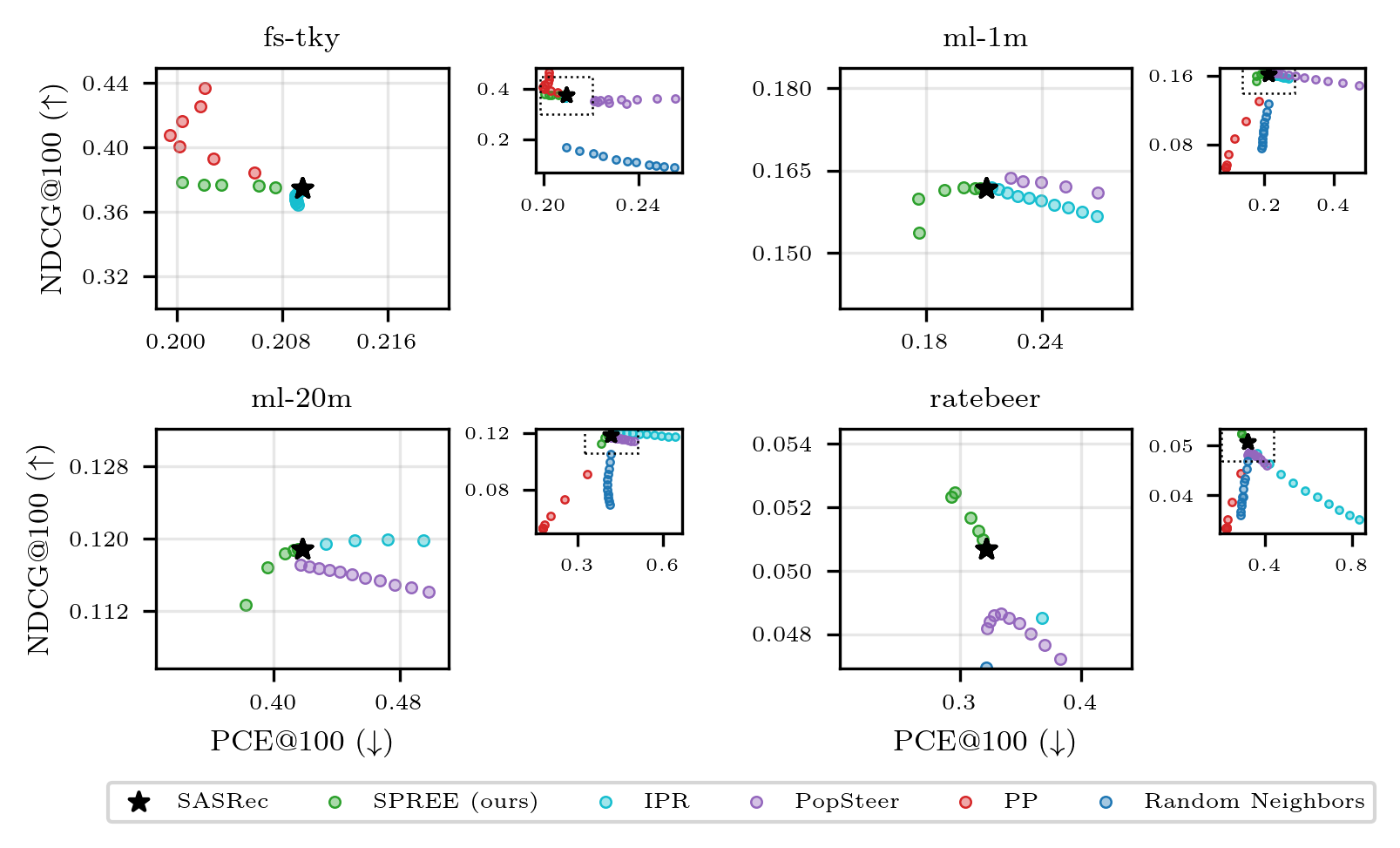
In Figure 3, only PP and SPREE consistently push PCE below the backbone, because both align with the user's history. PP pays for this with a steady drop in NDCG, except on fs-tky. Check-in data is highly repetitive, so sending users back to places they have visited is often right. SPREE largely keeps accuracy on fs-tky and ml-1m and even improves it slightly on RateBeer. Reading from the figure, on ml-20m at the strongest setting, SPREE's NDCG@100 drops from about 0.119 to about 0.112. IPR and PopSteer lower popularity across the board, losing a little NDCG while PCE goes up.
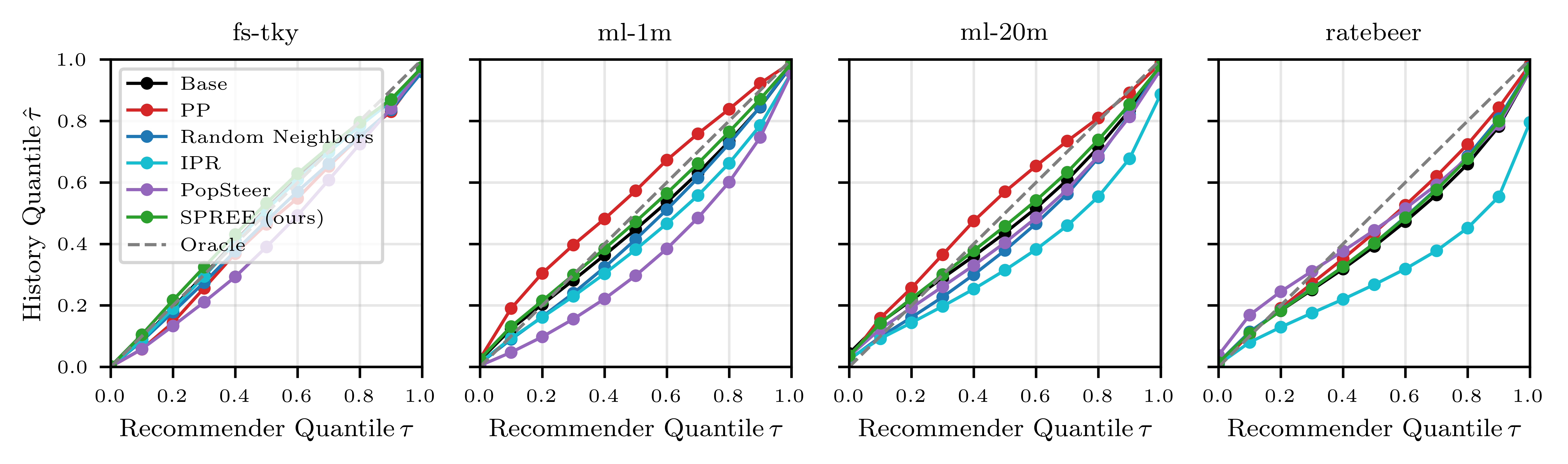
The calibration curves in Figure 4 also show direction. Apart from fs-tky, the backbone leans niche on the other three datasets. At the recommendation median quantile , the matching history quantile is about 0.45. In other words, these users on average like more popular items than the model gives them. Methods that lower popularity across the board make this bias worse. PP overcorrects on the two MovieLens datasets, leaning popular at every quantile. SPREE's curve stays closest to the diagonal.
The ablation is Table 4. Under the constraint that NDCG@100 drops by at most 10%, the largest is chosen, and versions with and without the estimator are compared.
| Dataset | PCE@100 backbone | SPREE | Without estimator | ALRP@100 backbone | SPREE | Without estimator |
|---|---|---|---|---|---|---|
| fs-tky | 0.210 | 0.200 (-4%) | 0.509 (+143%) | 4.663 | 4.713 | 3.636 |
| ml-1m | 0.211 | 0.176 (-16%) | 0.434 (+106%) | 6.339 | 6.337 | 5.883 |
| ml-20m | 0.418 | 0.382 (-9%) | 0.378 (-10%) | 9.012 | 9.017 | 8.912 |
| RateBeer | 0.321 | 0.293 (-9%) | 0.335 (+4%) | 5.652 | 5.860 | 5.577 |
ALRP (average log popularity) is the mean log popularity of recommended items and measures overall popularity. The version without the estimator does lower overall popularity, but it only improves alignment on ml-20m. On fs-tky and ml-1m its PCE more than doubles. SPREE keeps overall popularity nearly unchanged while PCE falls. This means it redistributes popularity among users. It gives more popular items to users who like popular items and more niche items to users who like niche items, while the total stays about the same.
Limitations as I see them
First, the experiments are small. The backbone is a 64-dimensional, 3-layer SASRec, and the largest dataset is MovieLens-20M. The authors are from Amazon Music, yet there are no music or online results. Whether SPREE works as well on large models or feature-rich industrial ranking models is still unknown.
Second, the estimator's quality varies. In Appendix Table 5, the Lasso R² is 0.638 on ml-20m but only 0.182 on fs-tky and 0.223 on RateBeer. That may be related to PCE falling only 4% on fs-tky. Also, itself can be computed directly from the user history and the recommendation list. The authors chose to predict it from internal representations instead. As I read it, the benefit is that the correction happens in a single forward pass, without first producing recommendations and then computing the bias; the cost is the uneven R² above.
Third, only the median is used. The bias signal uses a single point, , so each user gets just one coefficient that decides whether to push toward popular or niche items and by how much. The authors write in their limitations that this restricts targeted control to the center of the popularity distribution. After re-scoring and taking the top , the width of the distribution may change too, but the bias signal does not control that change directly, and the current method cannot specifically target the low- or high-popularity tail.
Fourth, the accuracy cost varies by dataset. Reading from Figure 3, on ml-20m at the strongest setting NDCG@100 drops by about 6%. The Table 4 results are also taken under a loose "at most 10% drop" constraint.
How a recommendation team could try it
- Start by diagnosing the existing model with PCE and the calibration curve. Compute PCE per user and plot the average calibration curve to see whether the bias leans popular, leans niche, or comes from a distribution that is too narrow. This step needs no model change and costs the least.
- If the bias really points in different directions for different users, try SPREE. Build two groups of artificial sequences from the 10% most and least popular items, and take the mean difference at the last layer as the direction.
- Skip the estimator at first. Use the true value of , computed once more after the recommendations are produced at inference time, to check the upper bound. Then decide whether training the Lasso estimator is worth it.
- Compare against the simplest per-user re-ranking. If re-ranking with the "niche score times user coefficient" described above gets the same effect, there is no need to touch the model internals.
Conclusion and assessment
The key lesson is that popularity bias should be measured and corrected per user. Measurement should compare whole distributions rather than just means. Correction can push toward popular items as well as toward niche ones.
| Dimension | Assessment |
|---|---|
| Problem importance | Medium to high. Popularity bias is widespread, and aligning with personal taste is closer to business goals than blanket de-popularization |
| Novelty | Medium. Quantile calibration and activation steering both have precedents; the novelty is combining them into per-user bias measurement and correction |
| Evidence | Medium to weak. Baselines are complete and the ablation is clear, but only small models and public datasets are used, with no online results |
| Engineering cost | Low. No retraining; it only needs contrastive sequences, one direction vector and a Lasso model |
| Worth trying? | Worth using PCE for diagnosis first; for the correction, compare against per-user re-ranking before changing model internals |
How did this read for you?
Hoot made a note. Thanks for the feedback.

One tap, no sign-in; tap again to undo. Only anonymous counts are kept, never who you are.
Discussion
Add experiment details, reproduction notes or a different take. Requires a GitHub sign-in.
Loading the discussion…