Contents · 8 sections
1What problem is it solving?2Why didn't routine checks catch it?3How much do conclusions change after the fix?4Too few epochs also changes the ranking5The unused text is the strongest signal6Limitations as I see them7How a recommendation team could use this8VerdictSHARE

Worth reading for anyone who evaluates recommenders, because the problem it uncovers is not in the models but in how the data files map onto each other. In HuggingBench, the public benchmark for recommending Hugging Face models and datasets, three of the four knowledge graphs that describe the items have their item IDs matched wrongly, so knowledge-graph recommenders have been reading another item's facts as this item's. The files pass the usual key and range checks; only a join by content reveals the mismatch. After the fix, every knowledge-graph method improves, with mean recall up by as much as 73%. The benchmark also ships each item's text description, which no reported method uses. Linear models that use this text train in minutes on a CPU and beat the best reported recall by 17%.
What problem is it solving?
HuggingBench was published at SIGIR 2025. The task is to recommend new resources to a user based on the models, datasets and Spaces they liked on Hugging Face. It has 38,624 users and 25,080 items, split per user into 60% training, 20% validation and 20% test. Besides the likes, it ships four external knowledge graphs that describe how items relate: one model is a fine-tune of another, a Space uses a given model, an organization publishes them.
Knowledge-graph recommenders (KGIN, KGCL, KGRec) rely on one convention: item i in the interaction file is entity i in the graph. They read both files by ID only and never look at names. A made-up example shows what happens when the convention breaks.
| ID | Item in the interaction file | Entity with the same ID in the graph |
|---|---|---|
| 0 | a quantized Llama variant | an image segmentation dataset |
| 1 | a Chinese QA dataset | a speech recognition Space |
| 2 | a speech recognition Space | a quantized Llama variant |
(Illustrative.) The model believes it is learning that item 0 is a quantized Llama related to Llama, but it is actually reading the relations of a dataset. The author joined the item list and the entity list by name. Only the homogeneous graph (item-to-item relations only) follows the convention. In the 1-hop and 2-hop graphs, none of the 25,080 items has the same ID as its entity; in the publisher graph, only 4 do.
Why didn't routine checks catch it?
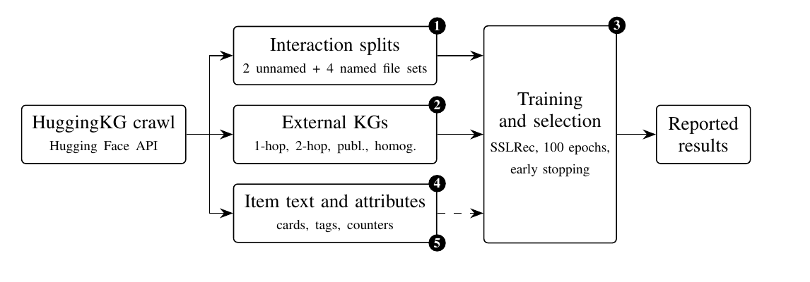
Every graph file set passes 34 key and range checks: contiguous IDs, unique names, disjoint splits, all IDs in range, and every item ID a legal entity ID. Each file is fine on its own; the error is in how two files correspond. It only shows up when the two lists are joined by name and the check asserts that item i equals entity i. The author groups the checks into six families. The first three cover clean splits, consistent encodings of the same data, and ID joins agreeing with name joins. Together they run 219 checks in 87 seconds on a CPU. On the released files only the "item i equals entity i" checks fail, with 75,238 violations.
There is also a clue to how it slipped in. The release encodes the same likes in six file sets, each with its own numbering. Between any two graph file sets, at least 25,077 of the 25,080 items have different IDs, and no mapping is shipped. Each graph was exported with its own numbering, which would explain how the mismatch went unnoticed.
How much do conclusions change after the fix?
The author reran every knowledge-graph method with the original hyperparameter grids and selection, over three random seeds.
| Method | 1-hop released | 1-hop corrected | Publisher released | Publisher corrected |
|---|---|---|---|---|
| KGCL | 0.1496 | 0.1591 | 0.1540 | 0.1604 |
| KGRec | 0.0845 | 0.1457 | 0.0943 | 0.1204 |
| KGIN (original code) | 0.1169 | 0.1445 | 0.1152 | 0.1475 |
(Test Recall@10, mean over three seeds, from Table V of the paper.)
Every method improves on every graph in every seed, by 4% to 73%, least for KGCL and most for KGRec. The homogeneous graph was aligned all along. After the fix, KGRec and KGIN beat it with every corrected graph in every seed, and KGCL with a corrected graph is on average within 0.0019 of it. The old ranking of graphs was skewed by whether their IDs lined up. The author counts 27 orderings: one method on different graphs, or one graph with different methods. After the fix, 10 of them flip in all three seeds. For example, on the 2-hop graph the original KGIN leads KGRec before the fix and trails it after.
In relative terms the gains fall mostly on rare items. Take KGRec on the 1-hop graph with 500 epochs and seed 42: for items with 1 to 4 training likes, the share of their test likes placed in the top 10 rises from 0.004 to 0.020, five times higher; for items with at least 100 likes it moves only from 0.148 to 0.155. Items with fewer than 100 training likes hold 54% of test likes. With misaligned graphs, most of the model's hits land on popular items. The aggregate metric is dominated by popular items anyway, so the error is hard to see in the total.
One question remains: does the fix help because an item gets its own facts, or just facts typical of its kind? The author runs a control: entities are shuffled and handed back to items, but only swapped among items of the same type (model, dataset or Space) whose number of graph facts falls in the same bin (0, 1, 2 to 4, 5 to 9, and so on). Each item thus gets someone else's entity of the same kind and similar information content. The correctly aligned graph beats every random assignment in every seed, and every random assignment beats the released graph. So an item's own facts help, and facts typical of its kind help too. The author notes this control cannot fully separate the two.
Too few epochs also changes the ranking
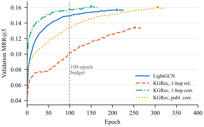
The protocol trains for at most 100 epochs and stops early after five evaluations without validation improvement. Early stopping only works if the cap is large enough. Recording the best epoch of 29 settings in each seed, the author finds that seven to eight settings hit the 100-epoch cap before early stopping fired. Raising the cap to 500 with everything else unchanged, 21 of the 23 truncated setting-seed pairs improve, with best epochs between 105 and 354, so this is not a matter of a few extra epochs. KGRec on the released 1-hop graph gains 31% in Recall@10. Comparing two methods at 100 epochs therefore partly compares how fast they converge.
The cap also inflates the cost of the misalignment. The model on the misaligned graph converges more slowly, so cutting at 100 epochs hurts it more. With 500 epochs, the gap between KGRec on the corrected and released 1-hop graph shrinks from 0.0613 to 0.0374 (mean over three seeds), though the corrected graph still wins in every seed.
The unused text is the strongest signal
Every item comes with text: type, name, tags, and the model or dataset card. None of the eleven reported methods uses it.
The author first tries EASE, a linear model with no side information. It learns an item-to-item weight matrix B that reconstructs each item's likes from the likes of other items, with the rule that an item cannot predict itself. The problem has a closed-form solution: one inversion of an items-by-items matrix, no iterative training. At recommendation time, summing the rows of B for the items a user liked gives every candidate's score. EASE alone reaches Recall@10 0.1684, above every reported, reproduced and corrected result.
Text enters by changing the matrix that gets inverted:
is the user-item like matrix, so counts how often two items are liked by the same users. is the text similarity matrix, whose entry (i, j) is the TF-IDF cosine similarity of items i and j, with zeros on the diagonal. is a weight chosen on validation data and the regularizer. One way to read this: two items with similar text look, in the matrix before inversion, as if they shared some users; their final weight in B is set by the whole inversion and is not guaranteed to be positive. The text is folded into the fixed B at solve time; scoring works exactly as before, with no similarity computed per request. With text similarity added, Recall@10 rises to 0.1846, 17% above the best reported result. All these linear models are computed in minutes on an 8-core CPU. Hoot says

- Two-item illustration: A has 4 likes, A and B share 1 user, and λ is 1. Without text, A's weight on B is 1 ÷ 5 = 0.2.
- With text: their similarity is 0.5 and w is 4, like 2 extra shared users. The weight becomes 3 ÷ 5 = 0.6.
- At scoring time, for a user who liked only A, B's score is the 0.6 in A's row.
With only two items, it can be worked by hand. Similar text acts like a few extra shared users. That boost is written into B during the inversion. Scoring never touches the text again. With many items, the whole inversion sets the weights, and they need not be positive. Source: the paper's EASE-with-text formula and Table VII; the two-item numbers are illustrative
| Method | Recall@10 |
|---|---|
| Best reported (KGCL, homogeneous graph) | 0.1578 |
| Best corrected knowledge-graph method (KGCL, publisher graph) | 0.1604 |
| EASE | 0.1684 |
| EASE + TF-IDF text | 0.1846 |
(From Table VII of the paper.)
A counterintuitive detail: given exactly the same input text, TF-IDF beats embeddings from bge-m3 and Qwen3-Embedding-0.6B in all four comparisons. The author's explanation is that hub text is highly templated. Two models from the same publisher have a median TF-IDF cosine of 0.40, against 0.03 for random pairs, so literal overlap in publisher and model names is itself a strong signal. Item type plus the organization/name identifier alone reaches Recall@10 0.1850, about the same as the full text at 0.1846.
Limitations as I see them
First, this is an audit of one benchmark, and the findings are verified on HuggingBench. Checks of other recommendation releases found incompatible numberings between releases of the same dataset, not the same misalignment.
Second, text is strong here partly because of the data: many items are quantizations and adapters of the same base model with near-identical names, which favors literal matching. In product or content recommendation, text may not be this strong.
Third, the random reassignment control keeps the degree distribution but not each item's exact structure, and the author says it cannot fully separate an item's own facts from structural effects.
How a recommendation team could use this
- Add a content-join check to offline evaluation data: join all items between interaction tables, feature tables and graphs by name or content ID once, and assert that IDs correspond. It takes seconds and catches mismatches that single-file checks miss.
- Log the best epoch of every run and rerun anything whose best epoch sits at the cap. Otherwise convergence speed leaks into model comparisons.
- Before a complex model, run a closed-form EASE baseline with text similarity. It takes minutes; if it already wins, the complex model's gains need a second look.
Verdict
Before trusting a ranking on a public benchmark, check that the data actually line up. The most useful part of this paper is not a new model but a reusable set of checks: join data files by content, look at best epochs, and try the simplest linear model on information nobody used.
| Dimension | Assessment |
|---|---|
| Importance | High. The misalignment underrates a whole family of methods and flips over a third of graph-configuration comparisons |
| Novelty | Medium. The checks are simple; the value is doing them systematically and measuring the consequences |
| Evidence | High. Three seeds, paired confidence intervals and a random-reassignment control |
| Engineering cost | Low. The checks run in 87 seconds; the linear baseline takes minutes on a CPU |
| Worth trying | Yes. Any evaluation set stitched together from several files can be checked this way |
How did this read for you?
Hoot made a note. Thanks for the feedback.

One tap, no sign-in; tap again to undo. Only anonymous counts are kept, never who you are.
Discussion
Add experiment details, reproduction notes or a different take. Requires a GitHub sign-in.
Loading the discussion…