Contents · 7 sections
1Five steps from scoring to choosing a depth2Decision models rank better, and the gain from graded labels nearly disappears3When a model reports over 90%, humans judged only about two thirds relevant4Why two parameters fix most of it5After calibration, the remaining gap comes from discrimination6In new domains, log loss falls but Brier is mixed7Using expected F1 to set the depth per questionSHARE

Ranking well does not make a model's reported relevance probability trustworthy; this paper checks the probabilities reported by LLMs and cross-encoders against TREC human relevance judgments and finds that two parameters remove much of the error, and that the repaired probabilities can decide how many documents to return for each question.
Take a RAG pipeline that retrieves, reranks and then cuts off the top few passages (illustrative): it does two things on every request. Take an illustrative question: a user asks "why are airplane windows round?" The system first takes 100 candidates with BM25, a reranker scores and sorts them, and then the top few are cut off and passed to the LLM. The ranking decides what the LLM reads first, and the cut decides how much it reads. Every extra passage costs context tokens, and irrelevant passages can distract the LLM's answer.
The hard part is how many to cut. A ranking score only tells the system that A ranks above B, not whether the passage at rank 4 is worth including. Suppose that among the window question's candidates only 3 actually explain the window shape, while another question has 30 relevant ones (illustrative). With a fixed top 10, the window question passes at least 7 irrelevant passages and the other question misses at least 20. To choose a depth per question, the system needs an absolute number: the probability that this passage is relevant. Only with it can the system estimate whether one more passage adds something useful or just adds noise.
The paper's two baselines are a fixed top k and a probability threshold fitted on a set of human-labeled data. A fixed depth ignores relevance probabilities; the threshold baseline uses them, but applies one global threshold to every question and has to be fitted on labeled data. Setting a depth per question requires relevance probabilities that can be trusted. Jev, released in September 2026, seems to provide them. Jev is a decision model: the caller gives it a judgment question, several relevance levels and a piece of content (here the user's query plus one candidate document), and instead of generating text it returns a probability for each level directly; adding the probabilities of the top levels gives the document's relevance probability. Its vendor, TypeSafe, promises that these probabilities are calibrated, meaning that among 100 documents the model scores at 80%, about 80 should actually be relevant.
Within weeks of their release, Jev and similar open-weight models were used as rerankers and for RAG evidence selection and claim verification, uses that act directly on the probabilities. Yet the existing independent calibration checks, one on text classification and one with binary labels, never compared these probabilities with graded human relevance judgments. Back to the window example: if Jev gives the passage at rank 4 a probability of 0.5, nDCG only cares that it ranks above the fifth passage and cannot say whether that 0.5 can be trusted.
This paper builds on an earlier work, Beyond Yes and No. That work had an LLM choose a relevance level for each document, used the model's probabilities (likelihoods) for the levels to compute an expected relevance as the ranking score, and left "whether these scores match human judgments" as future work. The authors first reproduce its ranking findings, then test the probabilities themselves with human labels from the TREC Deep Learning evaluations. The data are split by year into DL19 (labels from 2019), DL20 (from 2020) and DL21 (from 2021). The result: of the query-document pairs Jev scores above 0.9 on DL21, humans judged only 66% relevant. After fitting two parameters (a slope and an intercept) on 2,257 DL19 pairs and cutting by the corrected probabilities, Jev's mean F1 rises from 0.506 with a fixed top 10 to 0.638.
Five steps from scoring to choosing a depth
We keep using the airplane window question. The full pipeline runs like this:
| Step | Input | Operation | Output | Only at fitting time? |
|---|---|---|---|---|
| Retrieve candidates | query | BM25 takes the top 100 | Candidate documents | No |
| Score | query, one document, four relevance levels | The decision model returns one probability per level | The top two levels summed give this document's native probability | No |
| Fit calibration | DL19 native probabilities and human labels | Fit two parameters by maximum likelihood | a and b | Yes, once |
| Calibrate | Native probability, a, b | Apply a monotone map | Calibrated probability, document order unchanged | No |
| Choose depth | Sorted calibrated probabilities | Find the depth that maximizes expected F1 | Return k documents for this question | No |
The intermediate output of the scoring step looks like this (illustrative):
Question: How well does this passage answer the query?
Levels: Irrelevant / Related / Highly relevant / Perfectly relevant
Content: query=why are airplane windows round; passage=early airliners used square windows, and with cabin pressurization stress concentrated at the corners...
Returned: Irrelevant 0.01, Related 0.09, Highly relevant 0.40, Perfectly relevant 0.50
These four levels are the definitions TREC assessors use; Related means the document looks relevant but does not answer the question. The paper counts pairs with a human grade in the top two levels as relevant, so this passage's native probability is 0.40 + 0.50 = 0.90. A native probability is the one the model reports directly, before any correction. A cross-encoder has no level distribution; its native probability is its output logit passed through a sigmoid.
Decision models rank better, and the gain from graded labels nearly disappears
Before testing the probabilities, the authors confirm that these models really do rank well. The task is reranking the BM25 top 100 on 8 BEIR datasets, measured by nDCG@10.
The authors first reproduce the earlier work with the open LLM FLAN-UL2. All three findings hold in direction: graded labels beat the two-level "relevant / not relevant" labels, likelihood scoring beats parsing the label the model generates, and gains flatten beyond three or four levels. The absolute scores are 0.005 to 0.024 lower on average, and rerunning with the truncation length for each document raised from 256 to 512 tokens does not close the gap. So the earlier work's trends stand, but its reported absolute scores were not reproduced this time.
On the same candidates, asked with three relevance levels, Jev's mean nDCG@10 is 0.520, 0.046 above FLAN-UL2. It beats the cross-encoders MiniLM and bge by 0.050 and 0.034, but the strongest cross-encoder, monoT5-3B, by only 0.014, and leads on only 4 of the 8 datasets. The open 27B decision model pplx-decider scores 0.548, above Jev on all 8 datasets; the open 9B decision model Clef-flash scores 0.502. So the ranking leaders are the two decision models Jev and pplx-decider, an open model can rank ahead of Jev, and the 9B Clef-flash is about level with monoT5-3B.
The finding that graded labels beat two-level labels nearly disappears for decision models. Going from two levels to three, FLAN-UL2's nDCG@10 rises by 0.038, Clef-flash and pplx-decider by only about 0.006, and Jev even drops by 0.008. Jev's small drop depends on how ties are handled: its probabilities have only two decimals, so many documents tie, and breaking ties at random instead of by BM25 order turns the 0.008 drop into a 0.011 gain. For decision models, then, adding levels brings little, and the direction varies by model.
When a model reports over 90%, humans judged only about two thirds relevant
With ranking checked, the probabilities themselves come next. The authors use only pairs explicitly judged by TREC assessors: 2,257, 2,859 and 2,786 pairs for DL19, DL20 and DL21. Unjudged pairs have no human label and are left out. DL19 is used only for fitting, DL20 shares DL19's corpus, and DL21 is both a new year and a new corpus, MS MARCO v2.
Figure 1 is simple to read: the DL21 pairs are split into ten bins by the model's reported probability; the horizontal axis is the reported probability and the vertical axis is the actual share of pairs in each bin that humans judged relevant. A well-calibrated model gets out what it reports, so its curve should lie on the diagonal.
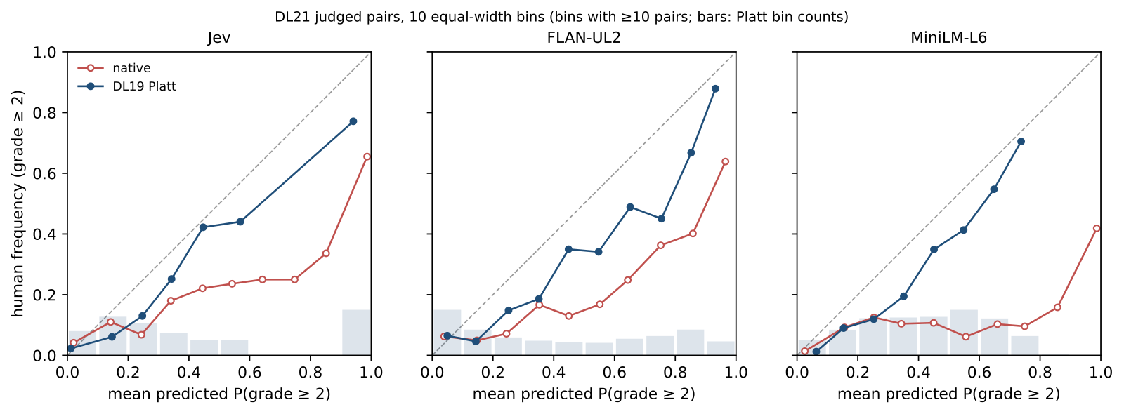
All three models' native curves lie well below the diagonal, meaning the actual share of relevant pairs is lower than the reported probability, so all of them are overconfident. Of the pairs Jev scores above 0.9, humans judged only 66% relevant; FLAN-UL2 is at 64% and MiniLM at 42%. By TREC human judgments, Jev's calibration promise does not hold, and the other models' native probabilities cannot be used directly as relevance probabilities either.
Jev has one more problem: it is the only model that returns exactly 0 or 1. Of DL21's 2,786 pairs, 1,006 got such an extreme value, and 158 of those contradicted the human judgment. Such errors matter because they are extremely costly in log loss. Illustration: for a pair humans judged irrelevant, if the model reports 0.9, the log loss is −ln(1 − 0.9) = −ln(0.1), about 2.3; if it reports 1, the paper clips the probability to 1−10⁻⁶ and the log loss is −ln(10⁻⁶), about 13.8.
So Jev's native log loss is 1.315, worse than FLAN-UL2's 0.783, even though Jev's Brier score and AUC are slightly better than FLAN-UL2's (the differences are not significant). The same model can rank in opposite order on different probability metrics, and systems that act directly on probabilities should watch out for the values 0 and 1.
Why two parameters fix most of it
If native probabilities are too high, one possibility is that the model's ranking is fine and only its values are shifted upward overall. In that case there is no need to switch models or retrain; a small map after the model is enough. The authors use Platt scaling: it first clips the native probability to [10⁻⁶, 1−10⁻⁶] (so values of exactly 0 or 1 still have a logit), then converts it to a logit, multiplies by a positive slope, adds an intercept and converts back to a probability:
is the native probability, the calibrated probability, and the sigmoid. The slope decides whether probabilities are spread apart or pulled toward the middle, and the intercept decides whether all probabilities shift up or down. With a positive slope the map is monotone, so document order is completely unchanged; it is fitted once on DL19 by maximum likelihood and then applied unchanged to DL20 and DL21.
Why two parameters; would an intercept alone not do? Illustration: logit(0.9) is about 2.2 and logit(0.1) about −2.2. Suppose 0.9 should be corrected to around 0.7 (logit about 0.84), while the 0.1 bucket is already roughly right. An intercept alone would have to subtract 1.36, dropping the logit of 0.1 to −3.56, a probability of about 0.03, pushed far too low.
With and (illustrative values), 0.9 becomes about 0.70 while 0.1 stays about 0.10. The slope lets the high and low ends be corrected separately, which a single intercept cannot do.
Applying these two illustrative values to the window question's 5 candidates:
| Passage (illustrative) | Native probability | Calibrated probability | Human grade |
|---|---|---|---|
| A: how rounded corners spread cabin pressure stress | 0.99 | 0.93 | Perfectly relevant |
| B: why airliners switched to round windows after square-window crashes | 0.99 | 0.93 | Perfectly relevant |
| C: square windows concentrate stress at the corners under pressurization | 0.90 | 0.70 | Highly relevant |
| D: the three-layer glass structure of cabin windows | 0.50 | 0.33 | Related |
| E: a buying guide for round windows in home decor | 0.10 | 0.10 | Irrelevant |
The order is unchanged; only the values change. Passage D looks relevant but does not answer the question, so by TREC's definition it counts as not relevant, which matters when choosing the depth.
The real results are read on four metrics, all on DL21 in the table below. Brier is the mean squared difference between the probability and the 0/1 label; illustration: reporting 0.9 contributes 0.01 if humans judged the pair relevant and 0.81 if not. ECE splits predictions into ten bins and averages the gap between the mean prediction and the actual share in each bin. AUC is the probability that a randomly drawn relevant pair scores higher than a randomly drawn irrelevant one; it only looks at order, so calibration cannot change it. Lower is better for Brier, log loss and ECE; higher is better for AUC.
| Model | Brier (native to calibrated) | Log loss (native to calibrated) | ECE (native to calibrated) | AUC |
|---|---|---|---|---|
| FLAN-UL2 | 0.237→0.171 | 0.783→0.514 | 0.248→0.124 | 0.831 |
| MiniLM | 0.476→0.188 | 2.373→0.554 | 0.503→0.108 | 0.766 |
| bge | 0.280→0.177 | 0.984→0.523 | 0.291→0.121 | 0.811 |
| monoT5-3B | 0.327→0.193 | 1.160→0.557 | 0.359→0.177 | 0.823 |
| Jev | 0.213→0.147 | 1.315→0.478 | 0.211→0.100 | 0.861 |
| Clef-flash | 0.202→0.172 | 0.596→0.519 | 0.212→0.115 | 0.836 |
| pplx-decider | 0.192→0.144 | 0.611→0.447 | 0.212→0.094 | 0.878 |
All three error metrics fell for every model on DL21, and on DL20 as well. Two parameters fitted on just 2,257 pairs still work on a new year and a new corpus. The correction is not complete: in Figure 1 the calibrated curves still sit slightly below the diagonal at high probabilities.
Jev was queried once per question through the API, and all of its numbers in the table come from that one result. To check whether one draw suffices, the authors resent the request three more times for 300 DL21 pairs, and Brier changed by at most 0.004, less than most gaps between models. So run-to-run variation of single API requests cannot explain most of the gaps in the table.
The wording experiment further shows that the error lies mainly in the scale of the values. Replacing the assessor-style question with the earlier work's two-level question raises Jev's native Brier from 0.213 to 0.322. After calibrating each on DL19, the two questions give 0.147 and 0.156, with similar AUC. Six other wordings give native Brier scores from 0.196 to 0.308, and after calibration they are at most 0.006 above the assessor question. Changing the wording mainly changes the size of the reported values, and calibration nearly erases that difference.
After calibration, the remaining gap comes from discrimination
After the same calibration, Jev's DL21 Brier is 0.023 below FLAN-UL2, 0.030 below bge and 0.046 below monoT5-3B. This advantage over the cross-encoders holds only on DL21; on DL20, bge and Jev differ by only 0.005, which is not significant. What can be said is that Jev was better on this year's held-out data, not that it always beats cross-encoders.
The open models split in two. The 27B pplx-decider has a calibrated Brier of 0.144, not significantly different from Jev's 0.147. The 9B Clef-flash matches Jev on DL20 (0.119 vs 0.123) but falls to FLAN-UL2's level on DL21 (0.172 vs 0.171). So an open 27B model can reach the same level of calibrated probabilities as Jev, while the 9B Clef-flash did not hold up on the new corpus.
To see where the gap comes from, ECE and AUC have to be read separately. After calibration, every model's ECE is between 0.094 and 0.124 except monoT5-3B at 0.177, so the accuracy of the values differs little. AUC keeps its original gaps: MiniLM 0.766, Jev 0.861, pplx-decider 0.878. The two models with the highest AUC also have the best calibrated Brier.
Once calibration brings every model's values to a similar level, the remaining advantage comes mainly from which model better separates relevant from irrelevant pairs.
In new domains, log loss falls but Brier is mixed
The authors apply the DL19-fitted parameters unchanged to four BEIR datasets. These datasets define grades differently from TREC, so the relevance threshold becomes a human grade of at least 1. Jev's log loss falls on average from 1.044 to 0.654, dropping on all four datasets, and it also drops for all three cross-encoders (MiniLM, bge and monoT5-3B).
Brier is a different story. Jev improves on TREC-NEWS and Robust04 and worsens on TREC-COVID and DBPedia-Entity, so its mean Brier over the four datasets rises from 0.197 to 0.214. With the TREC assessor-style question, FLAN-UL2's native probabilities were not very inflated to begin with, and adding the map worsens its Brier on all four datasets.
TREC-COVID is the worst case: this pair of parameters raises every model's Brier there except monoT5-3B's. The a and b learned on DL19 can lower the log loss of Jev and the cross-encoders in a new domain, but do not guarantee a lower Brier.
Using expected F1 to set the depth per question
Back to the opening question: how many passages should the window question pass to the LLM. F1 is defined as , where is the number of relevant documents among the returned and is the number of all relevant documents among this question's candidates. Neither is known online, but calibrated probabilities can estimate their expectations: a document's relevance probability is its expected contribution as a hit, so the sum of the top probabilities is the expected number of hits, and the sum over all candidates is the expected total number of relevant documents. Plugging these two expectations directly into the F1 formula gives the depth rule. The paper calls this a plug-in form: it maximizes the plugged-in approximation, not the exact expectation of F1, and "expected F1" below means this approximation.
The paper notes that this rule corresponds to an intuitive test: adding the next document pays off only if its probability exceeds half of the current expected F1. Because the bar is half of the current expected F1, each question gets a different bar, which is more flexible than one global threshold. Hoot says

Query A (illustrative)
- Documents
- 5
- Predicted probability each
- 0.8
- Sum of p
- 4 documents
- Actually relevant
- 5 documents
1 more than the sum of p
Query B (illustrative)
- Documents
- 5
- Predicted probability each
- 0.8
- Sum of p
- 4 documents
- Actually relevant
- 3 documents
1 fewer than the sum of p
Binned together (illustrative)
- Documents
- 10
- Mean predicted probability
- 0.8
- Sum of p
- 8 documents
- Actually relevant
- 8 documents
Observed share 0.8, matching the prediction
Illustrative numbers, not an experimental result. All 10 predictions are 0.8, so they share one bin, and the observed 8/10 matches the prediction: a reliability diagram sees no problem. Yet the sum of p gives 4 documents for both queries, while the actual counts are 5 and 3. A check that bins all pairs together cannot tell these cases apart, and this does not mean any model actually behaves this way.
Source
Numbers are made up for illustration; binning of all DL21 pairs is from the paper's Figure 1, and the use of the sum of p is from its expected-F1 truncation section.Illustration: a question has only 3 candidates, with probabilities 0.3, 0.3 and 0.25. The expected F1 of the top 2 is about 0.42, half of which is 0.21, so the third document at 0.25 is still worth including. With a global threshold of 0.30, the third document would be dropped.
Working through the window question's calibrated probabilities (illustrative, only 5 candidates listed): going down from the first passage, A, B and C each exceed half of the expected F1 at that point. All probabilities sum to about 3.0 and the top 3 to 2.56, so the expected F1 is about 2×2.56/(3+3.0), or 0.85, half of which is 0.43. Passage D's probability of 0.33 is below 0.43, so the cut stops at 3.
With native probabilities, the total is 3.48 and the top 3 sum to 2.88, so the expected F1 is about 0.89, half of which is 0.44. D's native probability of 0.50 is above 0.44, so D is included; with D, the expected F1 is about 0.90 and half is about 0.45, and E's 0.10 falls below it, so the cut stops there. By the human labels, cutting at 3 gives F1 of 1, and cutting at 4 gives 6/7, about 0.86. Overconfident probabilities make the rule cut too deep and pass passages that look relevant but do not answer the question to the LLM.
The rule cuts accurately only when the probabilities can be trusted, so it presupposes calibrated probabilities. The rule itself needs no tuned depth or threshold, but the two calibration parameters still have to be fitted on DL19's human labels.
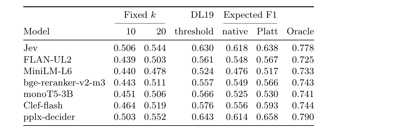
The real comparison is run on DL21, with unjudged documents removed before cutting. There are three control groups. The first is a fixed top 10 or top 20. The second is a probability threshold chosen on DL19 to give the highest mean F1, which keeps documents down the ranking and stops at the first one below the threshold (0.30 for calibrated Jev). The third is an oracle that uses human labels to pick each question's best depth, unavailable online and shown only as an upper bound.
Calibrated Jev cut by expected F1 reaches a mean F1 of 0.638, level with the tuned threshold's 0.630 and clearly above a fixed top 10 (0.506) and top 20 (0.544), though still short of the oracle's 0.778. A rule with no parameter of its own matches a threshold tuned specifically on labeled data, while fixed depths lose a lot.
For 5 of the 7 models, the expected-F1 rule matches or beats the tuned threshold; MiniLM and monoT5-3B do not, so the rule is good enough for most models but not every model can match the threshold.
Calibration raises F1 for every model. Jev rises from 0.618 with native probabilities to 0.638, and the mean number of documents returned per question falls from 28.6 to 26.1. This matches the direction of the window example: when native probabilities are too optimistic, the rule really does cut too deep.
With this rule, Jev's 0.638 and pplx-decider's 0.658 are both above the best of the three cross-encoders, 0.566. The lead in AUC also shows up in the F1 of the cut.
Back to the airplane windows: ranking puts A, B and C first, calibration changes D's 0.50 to 0.33, and the expected-F1 rule therefore keeps D away from the LLM. When this approach is deployed, the only human labels it needs are the 2,257 pairs used to fit a and b. On TREC the same parameters carry across years and corpora; in new domains, Brier goes up on some datasets and down on others.
How did this read for you?
Hoot made a note. Thanks for the feedback.

One tap, no sign-in; tap again to undo. Only anonymous counts are kept, never who you are.
Discussion
Add experiment details, reproduction notes or a different take. Requires a GitHub sign-in.
Loading the discussion…