Contents · 10 sections
1What problem does it try to solve?2Overall architecture3Step one: compress several behaviour sequences into one4Step two: use user and context features as "lenses" to reorganize the history5Step three: give HSTU attention linear complexity6Step four: summarization and compression7What the experiments show8Limitations as I see them9How a recommendation team could try it10Conclusion and assessmentSHARE

Teams working on long-sequence ranking and retrieval can read this one, focusing on two things: a diagnostic experiment of "add noise, remove noise" that costs almost nothing to reproduce, and an approximation that rewrites HSTU attention with linear complexity. The evidence for the main method itself is weak: there is not a single ablation row in the paper, and every number is a comparison against an unnamed production baseline. CMSL (Constructive Multi-Sequence Learning) comes from Meta, and its core idea in one sentence: instead of reading the user history as one sentence, at every layer use user and context features to re-express the same history from K angles as K sequences, run self-attention on each separately, then merge them back into one. The paper reports that on product surface 1, Eval NE drops 0.62% for comment prediction and 0.33% for likes; plugged into 3 other surfaces as an upstream user model, the drops range from 0.06% to 0.13%; used for retrieval, 4 online metrics rise 0.09% to 0.17%. Meta's internal convention is that an NE drop of 0.03% counts as significant.
What problem does it try to solve?
Most sequential recommenders today copy the LLM recipe: treat the user history as a string of tokens, feed it into self-attention, and predict the next one. The authors argue one part of this analogy does not hold. The words in a sentence follow on from each other, while a user history interleaves several interests, mixed with casual clicks and accidental taps. As an illustration: a user watches 5 Python tutorials in the morning, scrolls through 8 cooking videos at noon, and comes back to programming in the evening. The task is to predict whether they will comment on a new programming video. A single-sequence model has to spread its attention across these 13 items; the cooking videos, though barely related to the current prediction, still take a share of the weight, and may even lead the model to learn a spurious correlation such as "programming is related to cooking". The authors call this context pollution, borrowing the LLM observation that irrelevant content in a prompt drags down reasoning.
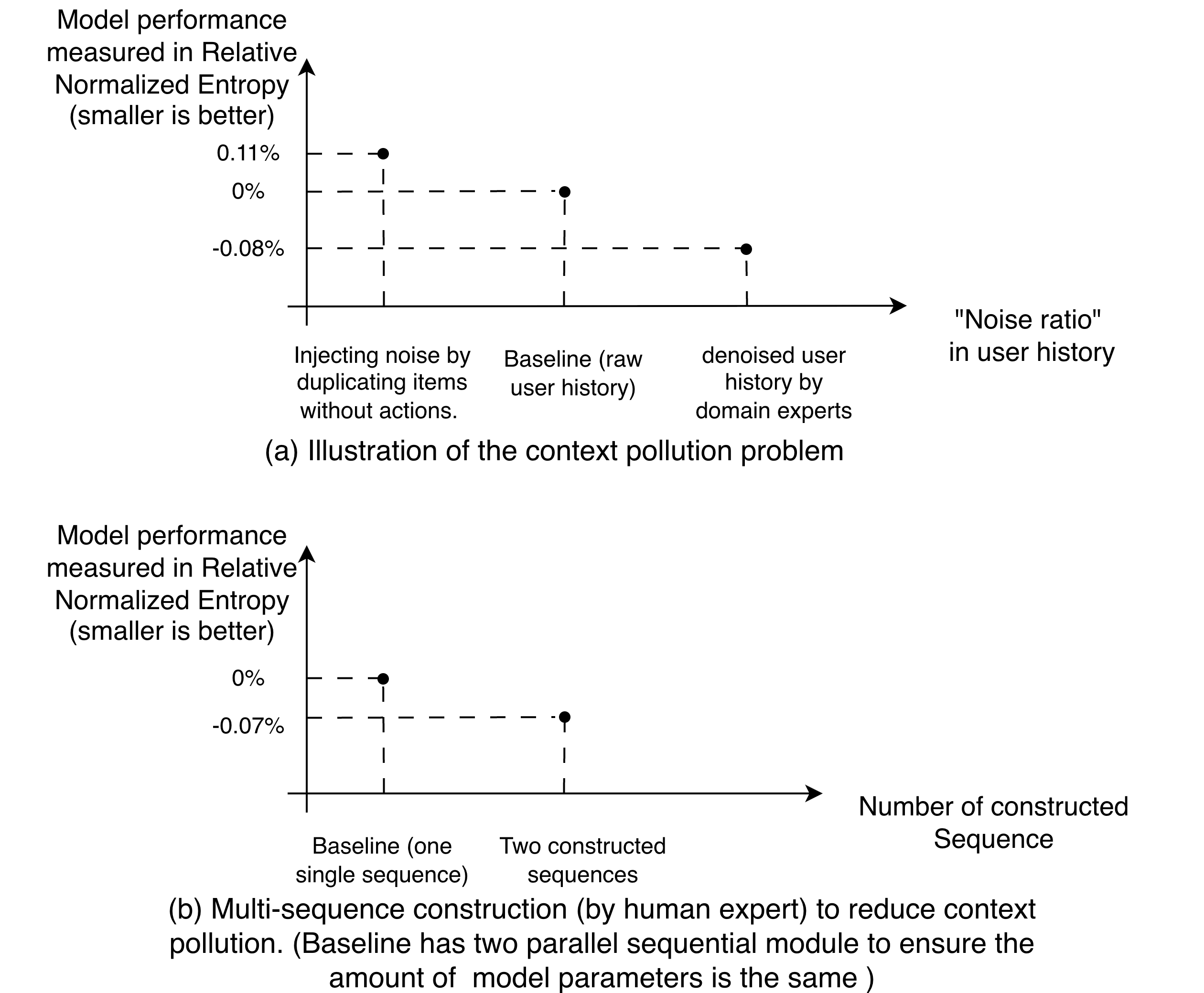
Figure 1 is the most convincing part of the paper. The top half shows that noise in the history really affects results: adding noise makes NE 0.11% worse; expert denoising makes it 0.08% better. The bottom half shows that "reading it split apart" helps in itself: a hand split into two sequences by experts beats the single-sequence baseline by 0.07%, and the baseline also has two parallel modules, so parameter counts are matched. Against the 0.03% significance line, all three gaps pass. Both the denoising and the split were done by hand by experts, so reproducing them means substituting your own rules, such as splitting by category or by surface. This shows the problem is real, and that it can be measured by changing only the input, without touching the model architecture.
A manual split cannot run in production: item IDs carry no meaning by themselves, and experts cannot split histories for billions of users one by one. CMSL's approach is to let the model learn how to split.
Overall architecture
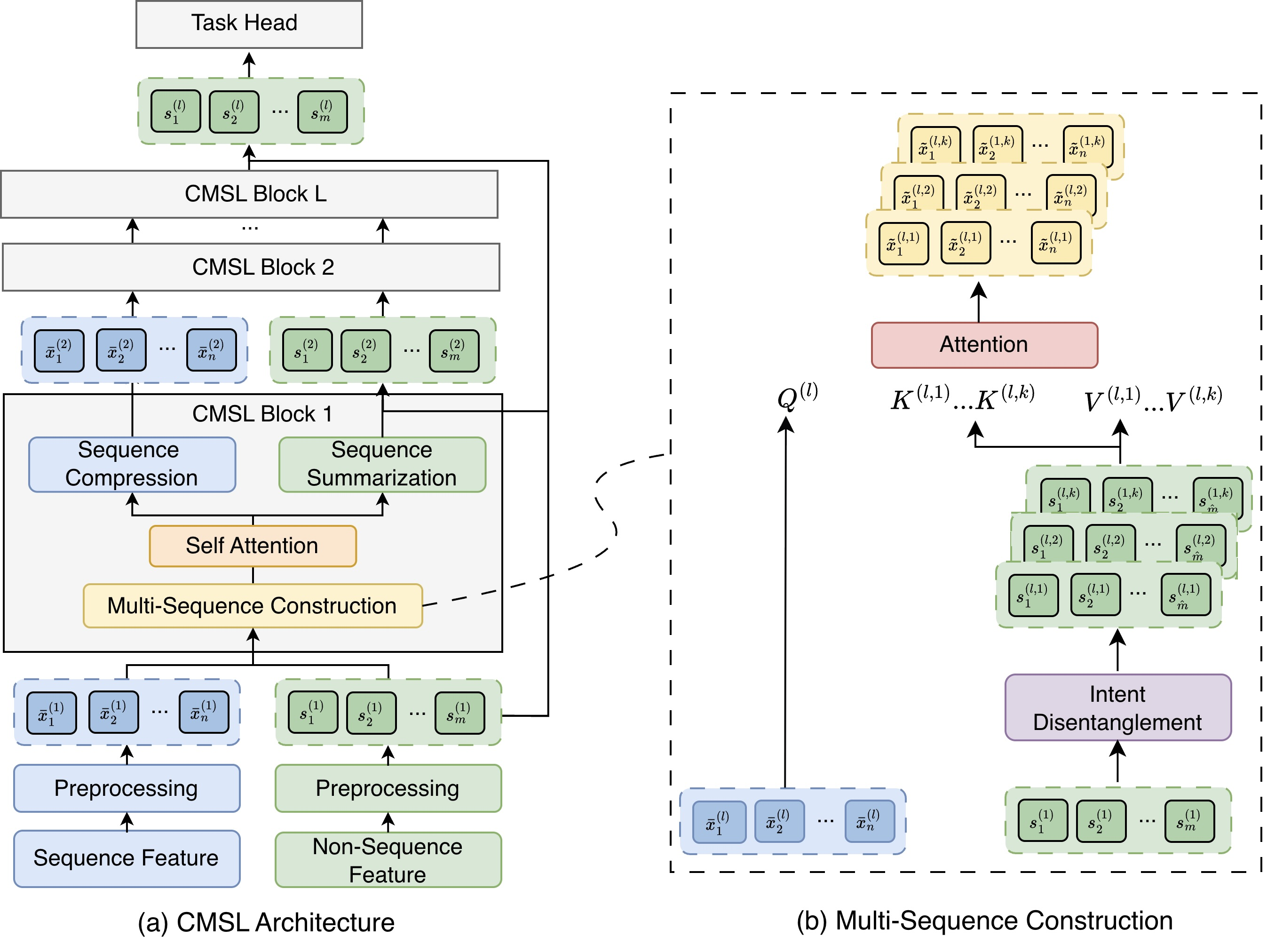
| Step | Input | What it does | Output |
|---|---|---|---|
| Sequence preprocessing | Several sequences on the same surface, such as clicks, likes and comments | Give each position of each sequence a score between 0 and 1, then take a position-wise weighted sum | One sequence (n positions, d dimensions each) |
| Multi-sequence construction | and non-sequence features | Split non-sequence features into K groups; each group runs one cross-attention with | K sequences, all of length n |
| Self-attention | Each sequence | Approximate HSTU attention on each separately | K sequences |
| Sequence summarization | Each sequence | Attention pooling with that group's non-sequence features as the query | K summary vectors, passed to the next layer |
| Sequence compression | K sequences | Concatenate along the feature dimension and pass through an MLP | One sequence, passed to the next layer |
The K summary vectors from the last layer are concatenated and handed to task heads such as CTR and CVR.
Step one: compress several behaviour sequences into one
Why is this step needed? On a social platform one user has many behaviour sequences, and running each through the model separately is too expensive. CMSL groups sequences with similar attributes, such as clicks, likes and comments on the same surface, and compresses each group into one: each sequence gets a small MLP that scores every position, , and the sequences are then summed position by position with those weights:
is the sigmoid, is the score of position in sequence , and is that sequence's embedding. In the formula every sequence in a group has n positions and position i is added directly, which requires the sequences in a group to be aligned by position already. Sequences of different lengths first have to be brought to the same n positions, for example by truncating each to its latest n items and zero-padding shorter ones; this step is yours to choose when reproducing. A hand-computed illustration: at position 3, the click sequence's embedding is with score 0.9 and the like sequence's is with score 0.5, so the weighted sum is . A sequence with a lower score contributes less at that position. Every later layer then processes only one sequence, at the cost of blending different behaviours at the same position.
Step two: use user and context features as "lenses" to reorganize the history
This is where CMSL really differs from single-sequence models. It has two sub-steps.
First, intent disentanglement. Non-sequence features such as user age, language and country code go through K projection heads, giving K groups of representations ; each group is then projected into a key and a value . Each group drawn on the right of Figure 2 has m vectors, as many as the input non-sequence feature vectors, so each group has m keys and m values, and the attention that follows distributes weight among these m vectors. The authors intend each group to correspond to one user intent.
Second, cross-attention. The sequence representation is projected into a query , which runs multi-head attention with each of the K key-value groups, giving K new sequences .
There is an easy misreading here. "Constructing multiple sequences" sounds like sorting the history's items into K buckets, but going by the formula, that is not what happens. All K sequences have length n, the same as the original. The query comes from the history and the keys and values come from non-sequence features, so the new vector at each position is a weighted sum of group k's non-sequence feature vectors, and the history items decide the weights. Back to the illustration: if group 1 has learned an intent leaning towards "work and study", the Python-tutorial positions match the related feature vectors in that group better and get more distinctive representations. If a cooking-video position matches every key in this group about equally, the weights are spread almost evenly, the resulting vector is close to the average of the group's m values, and different cooking videos get similar, poorly distinguished representations in that sequence. As I read it, this is more like viewing the same history once through each of K different lenses than cutting it into K pieces.
Step three: give HSTU attention linear complexity
Why is this step needed? The cost of self-attention grows with the square of sequence length, and constructing K sequences multiplies it by K. Meta's production systems commonly use HSTU attention, which has no softmax normalization:
is the causal mask. The authors start from the Taylor expansion of SiLU: . The first two terms involve only and , and the square of can be written as an inner product of the two vectors after each is expanded to dimensions. So defining , of length , lets the main part be written as linear attention : compute once and multiply each query by it, with no matrix. This is the unmasked form; with a causal mask, query i may only multiply the accumulated over the first i positions, and the usual linear-attention approach is a prefix sum along positions, which keeps the same order of cost. The expansion's error grows when is large, so the authors also wrote a sparse kernel that adds back the large entries of , written . The paper does not say how this sparse kernel in CMSL attention selects the large entries without computing the full ; it says only that the kernel is inspired by native sparse attention:
Two points need a literal reading here. First, the given in the paper's Equation 3 is exactly the form above, without coefficients, so by the source the linear part computes , which differs in its coefficients from the Taylor terms . To make the two agree, scale each linear component of by and each quadratic component by . Second, read literally, contains the large entries of themselves. But the linear part already covers every position, so adding the two counts the selected positions twice. The version consistent with the formula has store the difference at the selected positions and 0 elsewhere; this is my correction, not the paper's definition. As for how to pick the positions, my suggestion is to borrow the block idea of native sparse attention: score each block of keys by its mean against the query, keep the top-scoring blocks, and compute the exact value and the difference only inside them. This too is a reproduction plan, not what the paper specifies.
A hand calculation of when this pays off. Take , which expands to dimensions. At sequence length , the original attention takes about billion multiplications; the linear part first computes and then multiplies each query by it, about million in total for the two steps, a saving of just under 4x. At , the linear part takes about 68 million while the original attention needs only about 32 million, so it costs twice as much. This shows it saves compute only when the sequence is clearly longer than , and the expanded dimension grows quickly as grows.
The error bound in Equation 4 does not check out in one place. The authors write . Hand-compute : with the definition above, , while , so the inequality fails; even with the Taylor coefficients 1/2 and 1/4 the result is 0.75, still slightly above 0.73. The gap is larger for negative : at SiLU is about −0.14, while the quadratic gives 0.75. So the approximation relies mainly on the sparse correction term to fill in the large values, and anyone reproducing it has to measure the approximation error and the actual speed-up themselves.
Step four: summarization and compression
Summarization uses PMA (Pooling by Multi-head Attention, attention pooling over a sequence with a set of query vectors): with group k's non-sequence features as the query, attend over sequence k to get the summary . In standard PMA each query vector produces one output, so the size of is set by the number of queries and does not depend on the sequence length n; the authors call it a fixed-length vector. These vectors join the non-sequence features in the next layer. The paper does not say whether sequence summarization combines the summary vectors with the existing non-sequence features by concatenation, addition or replacement, so the number of vectors in the next layer's non-sequence input cannot be determined; what is certain is that the next layer's intent disentanglement takes into account what this layer read from the history. The authors' reasoning is that passing raw sequences directly between layers would carry the noise all the way through.
Compression keeps the number of sequences from multiplying by K at every layer: the K sequences are concatenated along the feature dimension and passed through an MLP, back to one sequence of length n and d dimensions. Stacking L layers this way, each layer takes in only one sequence.
What the experiments show
Training uses 128 H100s and 30 to 50 billion production samples per experiment. Ranking is measured by NE, lower is better; retrieval goes straight to A/B tests, because offline and online results often disagree for retrieval.
| Setting | How it is plugged in | Result |
|---|---|---|
| Surface 1 ranking | Train a CMSL model directly | Eval NE: comment −0.62%, like −0.33% |
| Surfaces 2/3/4 ranking | CMSL as an upstream user model whose user embeddings feed the production model | Eval NE: CTR −0.12/−0.09/−0.10%, CVR −0.10/−0.06/−0.13% |
| Surface 5 retrieval | U2U retrieval with CMSL user embeddings | 4 unnamed online metrics +0.092% to +0.171% |
The two ways of plugging it in were measured on different surfaces and different tasks, so the numbers cannot be compared directly. All 6 drops for the upstream approach lie between 0.06% and 0.13%, all above the 0.03% significance line. This shows that even when CMSL is used only as an asynchronously computed add-on user embedding, without touching the production model, it delivers significant gains, which is more practical for teams that cannot change their main model.
Limitations as I see them
First, there is no telling where the gain comes from. CMSL changes four things at once: multi-sequence construction, approximate attention, PMA summarization, and summary vectors fed back layer by layer. It is compared against a "production baseline" whose architecture is unknown. The only thing in the paper close to a control is the bottom half of Figure 1, but that is a manual expert split, not CMSL's learnable construction. Readers cannot judge how much of surface 1's 0.62% comes from multiple sequences and how much from the approximate attention making room for longer sequences.
Second, the key hyperparameters and costs have no numbers. What K is, how long the sequences are and how many layers there are appear only as symbols in the main text; how much compute the linear attention saves and how online latency changes are described only qualitatively. Other teams wanting to estimate migration cost have to measure everything from scratch.
Third, the 4 retrieval metrics have no names, and neither do surfaces 2 to 5, so improvements around 0.1% are hard to compare with other work.
How a recommendation team could try it
- First reproduce the Figure 1 diagnostic; this step does not change the model. Mix a batch of impressions without interaction into the user history and see how much NE worsens; then use a simple rule (such as by category or by surface) to split the history into two sequences with matched parameters and see whether it improves. If neither end moves, context pollution is not severe on your data and there is no need to go further.
- If the diagnostic shows a signal, add multi-sequence construction. Start with K=2, use existing user and context features as keys and values, add it to one layer only, and compare against a parameter-matched single sequence.
- Only bring in linear attention when sequences are very long; first compare its output with the original HSTU attention offline, then look at NE. By the hand calculation above, it is worth it only when the sequence is clearly longer than .
- If you want to run it upstream as an embedding, run the direct-replacement control on the same surface at the same time, to measure how much gain is lost in passing the embedding.
Conclusion and assessment
The key takeaway: noise and mixed interests in user history can be quantified first with three simple experiments, adding noise, removing noise and splitting by hand; once they are measured, consider letting the model use user and context features to learn how to split.
| Dimension | Assessment |
|---|---|
| Problem importance | High. Long-sequence modeling is the main line in ranking and retrieval, and mixed interests exist on almost every platform |
| Method novelty | Medium. Using non-sequence features as keys and values to reorganize history, and the polynomial-plus-sparse-correction attention approximation, are new; splitting multiple interests is an old direction |
| Experimental evidence | Weak. No ablations, unnamed baselines, no values for K or sequence length, and the error-bound formula does not survive a hand check |
| Engineering cost | Medium-high. You need a sparse attention kernel, and K sequences multiply each layer's compute |
| Worth trying? | Start with a diagnostic like Figure 1, which is very cheap; if there is a signal, add multi-sequence construction at small scale with K=2 |
How did this read for you?
Hoot made a note. Thanks for the feedback.

One tap, no sign-in; tap again to undo. Only anonymous counts are kept, never who you are.
Discussion
Add experiment details, reproduction notes or a different take. Requires a GitHub sign-in.
Loading the discussion…