SHARE

Retrieval and sequential-recommendation teams should read this, because it reframes the old question of how many vectors a user needs: instead of splitting interests with routing structures, it uses the training objective to force several prediction heads to each own a region of the catalogue, and it provides experimental evidence for why this does not collapse into one head. The Criteo and Sorbonne paper proposes COMPOTE (the authors' name, short for collapse-resistant multiple-hypothesis learning): a shared causal Transformer feeds M prediction heads; training starts with all heads learning together and gradually becomes "only the head that guessed best gets updated", and at inference each item is ranked by the highest cosine similarity across heads. On three Amazon 2023 review datasets it wins 11 of 12 metrics and beats the strongest generative baseline TIGER on NDCG@5 by about 9.7% on two datasets; at the same parameter count, giving the budget to one deeper head, training heads by plain averaging, or adding a routing gate all score lower.
A caveat: each of the three datasets has only about 25,000 items, metrics are offline Hit Rate and NDCG with absolute values between 2% and 9%, and the effect on catalogues of hundreds of millions of items and online traffic still needs your own validation.
What problem is it actually solving?
An example (illustrative). A user recently bought guitar strings and a tuner, then a console game. The next purchase might be guitar picks or a game controller, two items far apart in the catalogue.
| Approach | User representation | What ranks on top |
|---|---|---|
| Single-vector model | One vector, pulled by cross-entropy between the two item groups | Things that look like neither instrument nor game accessories |
| Multi-interest model | Several vectors assigned by routing or attention | Often all vectors point the same way, degenerating into one |
| COMPOTE | Three heads, each owning part of the catalogue | One head ranks instrument accessories, another game accessories |
The root cause is that the next-item distribution has several peaks. A single vector trained with cross-entropy settles between the peaks and aligns with none. Multi-interest models try to fix this with multiple vectors, but the authors' measurements show that without a dedicated training objective, the heads' directions coincide completely, which amounts to one vector.
The pipeline
| Step | Input | What it does | Output |
|---|---|---|---|
| Shared encoding | Last 50 item IDs | Item plus position embeddings through a few causal Transformer layers | Representation at the last position |
| M prediction heads | That representation | Each head is a small MLP producing its own vector | M query vectors |
| Scoring | Query and item vectors | Cosine similarity divided by a temperature, then softmax | One catalogue distribution per head |
| Training | The true next item | Annealed winner-takes-all loss, plus a small head predicting which head will win | Heads that each own a region |
| Inference | M sets of similarities | Take each item's highest, then sort | One ranked list |
The encoder is almost identical to a standard single-vector sequence model; the difference is all after the last layer: the shared trunk ends at the last position, then splits into M independent branches, which is what gives the heads room to divide the work.
How does training go from "learn together" to "winner takes all"?
The direct idea is winner-takes-all: for each sample, see which head gives the true item the highest probability and update only that head. In theory, which items each head handles can depend on the user's history. In experiments, each item's head assignment is almost fixed. During training, the model compares the heads' current probabilities for the true item and selects the winner again at every step, without fixing item assignments in advance. The problem is that a head that happens to lag early never wins, never gets updated, and is effectively dead.
So the authors smooth it with a temperature τ:
Here p is the probability head m gives the true item y. Each head's gradient weight under this loss is proportional to its probability raised to the power 1/τ. An example (illustrative): two heads give the true item 0.2 and 0.05.
| Temperature τ | Head 1 weight | Head 2 weight | Meaning |
|---|---|---|---|
| Very large | about 0.5 | about 0.5 | Both heads learn from this sample |
| 1 | 0.8 | 0.2 | Split in proportion to probability |
| 0.25 | about 0.996 | about 0.004 | Essentially only head 1 learns |
At τ of 0.25 the weights are 0.2 to the 4th versus 0.05 to the 4th, a factor of 256, so nearly everything goes to head 1. Training starts hot, so every head gets gradient and learns something; as the temperature falls toward 0, the loss becomes pure winner-takes-all, crediting only the best head per sample. The authors prove that if the soft assignment weights are held fixed during backpropagation, this loss gives exactly the same gradient as annealed multiple-choice learning from audio source separation. At high temperature, that objective weights the heads' cross-entropies nearly equally. As temperature tends to zero, it approaches the best head's loss. What is new is how to combine the heads at inference.
There is also a small head outputting M numbers between 0 and 1, the m-th being the probability that head m wins this sample. Labels follow the current result: the head giving the true item the highest probability is labeled 1, the others 0, and each output gets its own binary cross-entropy. This loss is weighted and added to the total, and its gradient flows into the shared encoder, effectively asking the encoder's representation to tell which head should be responsible; ranking at inference does not use it. The authors find it stabilizes training; without it Scientific NDCG@5 is 1.82, and with the best weight it reaches 1.92, so it helps but is not essential.
Why can inference skip the softmax?
Training applies a softmax over the whole catalogue per head; doing the same at inference would mean scanning the full catalogue per user, ruling out vector databases. The authors instead use cosine similarity directly: an item's score is its similarity to the head it is most similar to, then sort.
This works if each head's softmax normalizer is about the same size. After taking logs, "the largest softmax probability" equals "the largest similarity minus that head's normalizer", and when normalizers are equal, subtracting them does not change the order. On Game the three heads' normalizer distributions nearly overlap, concentrated between 12.2 and 15. Measurements agree: NDCG@5 with softmax is 4.01 and with raw cosine also 4.01. This means each head is an ordinary vector search at deployment, with M heads retrieved and merged by highest score, the same engineering shape as multi-interest retrieval.
The authors also prove that at a population WTA (winner-takes-all) optimum, scoring each item by its highest probability across heads preserves the true distribution's ranking. If the heads' softmax normalizers are equal, scoring by the highest cosine similarity gives the same guarantee. The one exception is when two items both have true probability at least 1/M. An example (illustrative): with M of 3 and two items at true probabilities 0.4 and 0.35, both above one third, the optimum has two heads each put all their mass on one of the items, both score a full 1, and they cannot be ordered. The larger M is, the smaller 1/M, and the more likely such ties are, which is the theoretical reason M cannot grow without limit.
Results
Experiments use three Amazon 2023 categories: instruments, industrial and scientific, and video games, each with about 25,000 items, histories truncated to 50, and the last action as test. Evaluation ranks the full catalogue rather than sampled negatives, so numbers are lower than in many papers but closer to real retrieval. Baselines include 7 ID-only sequential models, the generative model TIGER (generating the next item's Semantic ID token by token), and 6 multi-interest models.
| Method | Instrument NDCG@5 | Scientific NDCG@5 | Game NDCG@5 | Game Hit@10 |
|---|---|---|---|---|
| SASRec | 2.13 | 1.50 | 3.31 | 8.47 |
| TIGER | 2.44 | 1.75 | 3.66 | 8.68 |
| SINE (best multi-interest model) | 1.52 | 1.21 | 2.77 | 8.80 |
| COMPOTE | 2.45 | 1.92 | 4.01 | 9.26 |
Using only item IDs and one forward pass, COMPOTE beats TIGER, which uses item text and beam search. The multi-interest models are more telling: SINE (activating a few interests from a shared concept pool) nearly matches COMPOTE on Game Hit@10 but is 31% lower on NDCG@5, meaning its interest vectors widen the candidate pool without putting the target at the top.
Where does the gain come from? The authors run three controls with the same parameter count and encoder.
| Control | What it does | Game NDCG@5 | Mean cosine similarity between heads |
|---|---|---|---|
| Deeper single head | Give the parameters to one deeper head | 3.78 | Only one head |
| Averaged training | Every head updated equally on every sample | 3.78 | 1.00 |
| Routing gate | Learn a gate picking one head per sample | 3.78 | 1.00 |
| COMPOTE | Annealed winner-takes-all | 4.01 | 0.58 |
The last two controls' heads coincide exactly, a cosine similarity of 1, meaning they collapsed into one head; COMPOTE's three heads are clearly apart. So the gain comes not from more parameters, ensembling or routing, but from a training objective that makes the heads truly divide the work.
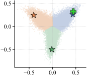
How complete is the division? On Game, two heads' top-10 lists have a mean Jaccard overlap of only 0.008, and 91.8% of retrieved items are reached by only one head; each head keeps 91.5% to 93.7% of its probability mass in its own region, and each head wins about a third of samples. This shows the heads are not subtly complementing each other but splitting the catalogue into nearly disjoint, fairly balanced blocks.
A more intuitive number: if you knew the target and picked the best head each time, NDCG@5 would rise 53%, 83% and 94% on the three datasets. Averaged training and routing gain nothing from the same trick, because their heads are identical. This proves the heads hold complementary information and shows the max merging rule leaves a lot of room.
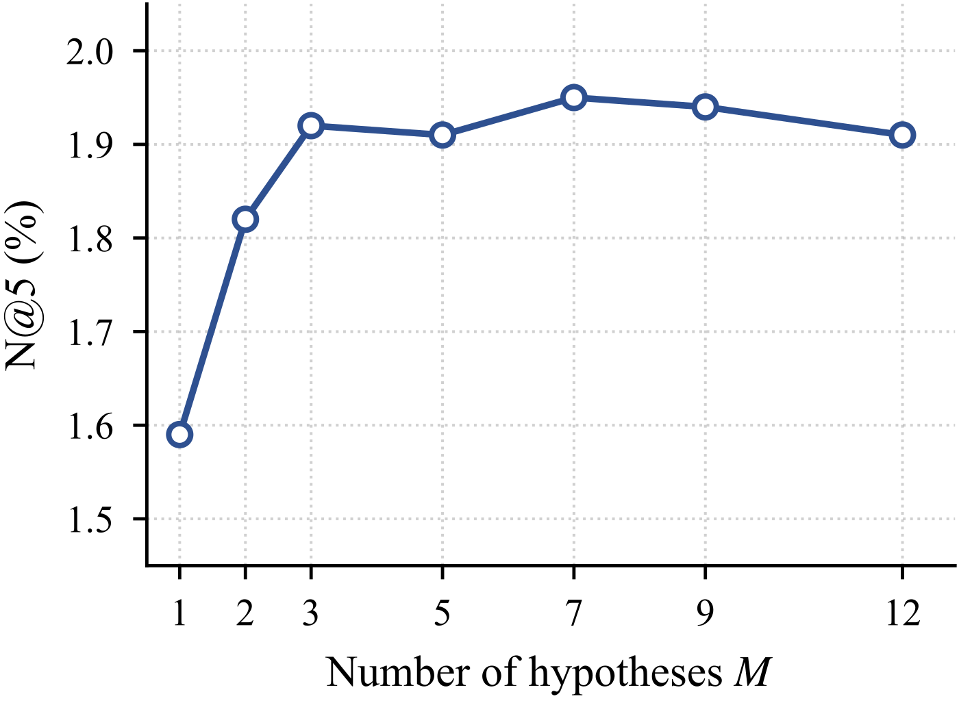
On head count, NDCG@5 rises from 1.59 at M of 1 to 1.92 at 3 and stays flat up to 12. This matches the authors' generalization bound: the number of heads affects overfitting risk only logarithmically, so a few more heads do not hurt noticeably, but bring no further gains.
Limitations as I see them
First, the scale is small. Each dataset has about 25,000 items and at most 95,000 users, with Hit@10 of only 4% to 9%. Industrial retrieval often covers tens of millions to hundreds of millions of items; whether a three-way split stays balanced at that scale, or needs dozens of heads, has to be tested on your own data.
Second, the merging rule is far from its ceiling. Picking the head with knowledge of the target lifts NDCG@5 by 53% to 94%, and the current max rule captures only a small part of that. Comparing scores across heads currently relies on normalizers happening to be close; under another data distribution that premise may fail, so check the normalizer distributions first.
Third, there are no online or latency numbers. M heads mean M vector searches plus a merge, roughly M times the retrieval cost of one vector; the paper evaluates only offline full-catalogue ranking, and the multi-interest baselines were retrained by the authors under one protocol.
How a retrieval team could try it
- Start with the cheapest diagnosis: if you already run multi-interest retrieval, compute the mean cosine similarity between interest vectors. Close to 1 means they have collapsed and the extra vectors only waste retrieval cost.
- Add 3 MLP heads on top of the user tower of your existing two-tower model, switch to the annealed winner-takes-all loss with temperature falling from high to low, and leave the rest unchanged.
- In serving, run one vector search per head and merge by highest similarity with deduplication; check that the heads' normalizers are close before dropping the softmax.
- Start with 3 heads rather than many; in the paper gains stop after 3.
Verdict
The key takeaway: multi-interest retrieval often lacks not more vectors but a training objective that makes the vectors divide the work; annealed winner-takes-all achieves it, and the inference shape fits existing vector search.
| Dimension | Assessment |
|---|---|
| Problem importance | High. Handling multi-peaked interests is a common weakness of single-vector retrieval |
| Method novelty | Medium. The loss comes from annealed multiple-choice learning in audio separation; the novelty is applying it to recommendation with a merging rule and theory |
| Evidence | Medium. Clean controls and a direct collapse measurement, but only offline metrics on three small datasets |
| Engineering cost | Low to medium. Changes are confined to the top of the user tower and the loss; the cost is M times the searches |
| Worth trying | Yes, especially for teams with multi-interest retrieval that suspect vector collapse |
How did this read for you?
Hoot made a note. Thanks for the feedback.

One tap, no sign-in; tap again to undo. Only anonymous counts are kept, never who you are.
Discussion
Add experiment details, reproduction notes or a different take. Requires a GitHub sign-in.
Loading the discussion…