Contents · 9 sections
1What problem does it actually solve?2Overall pipeline: the teacher only appears during training3How does the teacher score each chunk?4How does the student learn these scores, and why keep a contrastive loss?5Two new benchmarks: finding supporting chunks, not only the answer6What do the results show?7Limitations8How a search team could try it9ConclusionSHARE

Teams that build retrieval for RAG should read this paper. It changes a rarely questioned assumption in contextual embedding training: that a question has exactly one relevant chunk in a document. When RAG splits long documents into chunks, answering a question often needs more than the chunk that states the answer. It also needs the chunks that say which product or which year the answer is about. Current contextual embedding training accepts a single gold chunk and treats every other chunk of the same document as a negative, so these supporting chunks get pushed down. The core idea in one sentence: a query-aware compression model scores every token of the document, a chunk's score is the mean of its top few token scores, and the embedding model learns to fit these graded scores, with no answer-chunk labels needed. On the authors' new diagnostic benchmark, the 9B model finds the answer in its top 10 chunks for 45.5% of queries, against 31.1% for the strongest baseline, voyage-context-4. Dropping the distillation step and training only with contrastive loss lowers the answer-chunk hit rate on real search queries from 86.3% to 71.1%.
What problem does it actually solve?
Take the paper's own example. A property company holds thousands of leases that are almost identical and differ only in tenant, date and address. A user asks "what is the current monthly rent for 5 Park Avenue". The sentence that answers it, "the monthly rent is X", appears in every lease. The address that tells you which lease it is sits far away in the same document.
After chunking, a few chunks of one lease look like this (illustrative):
| Chunk | Content | Role for this question | How single-gold training sees it |
|---|---|---|---|
| A | "The premises are located at 5 Park Avenue" | Identifies the lease | Negative |
| B | "Rent is adjusted yearly from 2025" | Says whether the answer is current | Negative |
| C | "The monthly rent is X" | Answers directly | The only positive |
| D | "Property management contacts" | Irrelevant | Negative |
When only C is positive, the model learns to push A and B down, yet the reader or downstream LLM needs exactly A and B to confirm that C belongs to this lease and is the current rent. Plain chunk embeddings are worse still: encoded alone, C has no idea which address it belongs to, and the C chunks of thousands of leases look the same.
Contextual embeddings were designed for that second problem. The whole document is encoded in one pass, so each chunk vector carries information from the full text, and C's vector knows about Park Avenue. This paper targets the first problem: the training signal accepts only one answer chunk, and evaluation only checks whether that chunk ranks first, so supporting chunks like A and B are ignored on both ends.
Overall pipeline: the teacher only appears during training
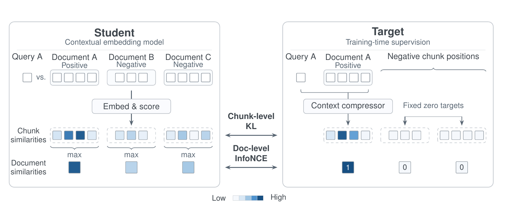
There are four steps:
| Step | Input | Output |
|---|---|---|
| 1. Chunk and encode | A document, with a chunking strategy sampled per batch and separator tokens between chunks | One context-aware vector per chunk |
| 2. Teacher scoring | The query and the positive document | A keep probability per token, pooled into a score per chunk |
| 3. Chunk-level distillation | Teacher chunk scores and student chunk similarities | The student's within-document ranking follows the teacher |
| 4. Document-level contrast | Each document scored by its best chunk | The positive document ranks above the other documents in the batch |
The student's data flow is simple. The whole document goes through the model once, and each chunk vector is the mean of its token vectors. The query is encoded alone by the same model, also as a token mean, and the dot product of the two is the similarity. The division of labor is the key point: the teacher decides which chunk inside a document should rank higher, and the contrastive loss decides which document should rank first. At inference the teacher is gone. The model outputs one vector per chunk as usual, the index is the same size as a plain chunk index, and there is no extra reranking stage.
How does the teacher score each chunk?
The teacher is the context compression model already running in Perplexity's answer pipeline. Its normal job is to take a retrieved document, keep only the spans relevant to the query, and pass those to the generator to save tokens. It is a cross-encoder that reads the query and the document together and outputs a keep probability between 0 and 1 for every document token.
The compression model was itself trained from sentence labels produced by an LLM in three classes. A sentence that answers the question on its own has target 1, and an irrelevant sentence has 0. A sentence that provides context needed to interpret the answer is mapped, as a class, to one shared soft target between 0 and 1. The LLM only assigns the tier and does not score each sentence. Each token's target is the average of the sentences it overlaps, weighted by overlap. This three-tier supervision teaches the teacher to tell answers, support and noise apart. What it actually outputs is a continuous keep probability per token, usually highest for answers, middle for support and lowest for noise. Chunk scores are computed from these continuous probabilities, and such graded scores are exactly what single-gold labels are missing.
Why score tokens rather than chunks? Because chunk boundaries are only decided at training time. A chunk's score is the mean of its 16 highest token scores, so one short key sentence is enough for a high score and is not diluted by filler. Because of this, whether you split by sentence or by 128 tokens, the chunk score can be computed on the spot without relabeling the corpus. The paper uses this to sample a different chunking strategy for each batch. The teacher is also far cheaper than calling a large LLM, so targets can be computed online for every batch.
For the lease (illustrative), the teacher might give C 0.9, A 0.6, B 0.5 and D 0.05. The old target was 1 for C and 0 for everything else. The new target gives A and B substantial credit.
How does the student learn these scores, and why keep a contrastive loss?
The chunk scores of the positive document are divided by a temperature and passed through a softmax, and chunks of other documents get probability zero. On the student side, the similarities between the query and every chunk of every document in the batch also go through a softmax. Training pulls the two distributions together with KL divergence:
Here is the teacher's chunk distribution for query i, is the student's, and is the number of queries in the batch. The intuition is that the student must learn not only which chunk is best but how far behind the second and third chunks are.
Working through the lease (illustrative, temperature 0.1 for easy arithmetic; the paper uses 0.075): scores of 0.9, 0.6, 0.5 and 0.05 become 9, 6, 5 and 0.5. After the softmax, C takes about 0.94, A about 0.05, B about 0.02 and D almost nothing. Compared with the C-only target, A and B are no longer forced to zero. They are only ranked behind C.
Because the teacher puts zero mass on other documents, this KL splits into two parts. One part asks the student's distribution inside the positive document to match the teacher. The other pushes the student's mass toward the positive document and away from others. So distillation already carries some document-level signal.
Why add a separate document-level contrastive loss, then? The paper defines a document's score as the similarity of its best-matching chunk and applies InfoNCE within the batch so the positive document ranks above the rest. The gradient only reaches the best chunk, so supporting chunks of the same document are never treated as negatives. The total loss weights distillation 1 and contrast 2.
The ablation shows what each part does:
| Training objective | Q2D-Chunk Answer@10 | ConTEB nDCG@10 | ViDoRe-V3 text nDCG@10 |
|---|---|---|---|
| Contrastive only | 71.1 | 68.1 | 58.7 |
| Distillation only | 85.8 | 82.4 | 60.3 |
| Both | 86.3 | 82.7 | 60.9 |
With contrast only, chunk retrieval falls by about 15 points on both chunk-level benchmarks, which means chunk-level distillation is the main source of finding the right chunk. Distillation alone keeps most of the document-level quality, and the contrastive term adds a little on all three benchmarks.
Two new benchmarks: finding supporting chunks, not only the answer
The older ConTEB benchmark labels one correct chunk per query and only rewards ranking it first. The authors built two new benchmarks that label both answer chunks and supporting chunks.
context-bench is a controlled diagnostic set. The authors adversarially inject content into long documents, for example a batch of leases that differ only in tenant and date, split them into sentences, and give each query a single correct document. It tests three things: picking the right document among near-duplicates, finding answer sentences whose meaning depends on context, and finding the supporting sentences that confirm the answer. It was evaluated blindly by the partner turbopuffer.
Q2D-Chunk comes from real search traffic. The authors take search queries longer than 100 characters from production logs. Long queries are more likely to have answers spread across a page. An LLM then rewrites each one into a full question. Pages are split into 128-token chunks, with answer and supporting chunks labeled. The median page has 4 answer chunks. Adjacent answer chunks count as one run, so these form 3 runs, and the stretch from the first run to the last spans about 45% of the page, which shows that answers rarely sit in one chunk. Because long queries often copy the page's wording, the authors also add three rewordings: a paraphrase with fewer shared keywords, an indirect form that replaces named entities with descriptions, and a first-person forum-post scenario.
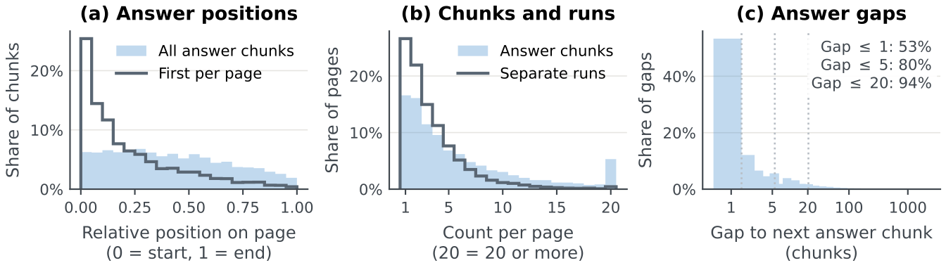
The figure explains why the benchmark is built this way: answers to real queries are often scattered across a page, and a benchmark that labels one answer chunk misses the rest.
What do the results show?
Main results (in %). Answer@10 works like this: each query is split into answer groups, one per part it asks about, and the score is the fraction of groups covered by the corpus-wide top 10 chunks, averaged over queries. context-bench has one answer group per query, so there it is simply a hit rate.
| Model | context-bench Answer@10 | Q2D-Chunk base | Q2D-Chunk indirect | Q2D-Chunk all evidence found |
|---|---|---|---|---|
| pplx-embed-v2-context-9b | 45.5 | 86.4 | 82.6 | 37.5 |
| pplx-embed-v2-context-0.6b | 21.9 | 83.1 | 77.3 | 35.2 |
| voyage-context-4 | 31.1 | 83.9 | 80.2 | 33.1 |
| pplx-embed-context-v1-4b | 26.4 | 74.9 | 65.4 | 33.1 |
| Nemotron-3-Embed-8B (no context) | — | 73.6 | 68.1 | 39.8 |
On context-bench the 9B model leads voyage-context-4 by 14.4 points, and the non-contextual voyage-4-large reaches only 6.4%. This shows that among thousands of near-identical documents, chunk vectors without document context almost never find the answer sentence.
On Q2D-Chunk the gap is much smaller. The 9B model leads voyage-context-4 by 2 to 3 points and its own previous generation by 11 to 17 points. Real queries often repeat the page's wording, which makes the task easier for everyone. With indirect queries every model drops, but the 9B model stays on top. The 0.6B model is 0.8 points behind voyage-context-4 on base queries but ahead on evidence and on tokens needed to cover all answer and evidence groups, a useful signal for teams that want a small model.
One result matters for deployment. If the same 9B model outputs a single vector per document, its document hit rate in the top 10 on context-bench drops by 29.8 points compared with ranking by the best chunk, while on Q2D-Chunk the two differ by less than one point. This means chunking is what finds the right document when you must pick one among many near-duplicates, and collapsing ordinary web pages into one vector costs little.
The authors also test visual document retrieval on ViDoRe-V3. The 9B model is trained only on text, but its backbone is a vision-language model that can read page images. To chunk a page, its visual tokens are split row by row into horizontal bands with the same separator token between them, and each band's tokens are averaged into one vector. Encoding page images this way, the 9B model beats Qwen3-VL-8B with one vector per page, and with 2 bands per page it beats Nemotron-3.5-8B with a 4x smaller index. This means one model can serve text and image pages from a single index.
Limitations
First, supporting chunks remain hard to find. Q2D-Chunk labels several evidence groups per query, each one piece of context needed to read the answer, such as which entity or period it belongs to, the condition under which it holds, or a unit or definition. A group counts as found if any of its chunks is retrieved. With answer chunks removed from the ranking and the top 10 chunks inspected, the share of queries with every evidence group recovered is 37.5% for the 9B model, and the best is actually the non-contextual Nemotron-3-Embed-8B at only 39.8%. The authors suspect that evidence chunks share many words with the query, which favors models without context. So the new training mostly improves finding the answer and the right document, and only partly solves supporting evidence.
Second, the teacher is not public. The method depends on Perplexity's production compression model, which was trained on three-tier LLM sentence labels. Another team would first have to train a similar token-level relevance model, and the paper does not count that cost.
Third, both new benchmarks were built by the authors' side. context-bench was scored blindly by turbopuffer, but its query types were designed around turbopuffer's customer needs, and Q2D-Chunk comes from the authors' own search traffic. Margins on these benchmarks may not carry over to other query distributions, and on real traffic the lead over voyage-context-4 is only 2 to 3 points.
How a search team could try it
- Measure the problem on your own corpus first. Sample production queries, label answer and supporting chunks by hand or with an LLM, and check how often current retrieval recovers the supporting chunks. If that rate is already high, there is no need to change training.
- Build the cheapest teacher. Instead of training a compression model, have an LLM label each sentence as answer, support or irrelevant, pool those into chunk scores, and replace single-gold labels with distillation on a small dataset. Compare Answer@10 and evidence recall before and after.
- If that works, train a token-level relevance model as an online teacher, so each batch can sample a different chunking and you can find the right chunk length for your corpus.
- Before launch, watch two things: the correctness of downstream LLM answers, and the number of tokens fed to the LLM to cover every answer and piece of evidence, which directly sets cost.
Conclusion
The key lesson: training labels for RAG retrieval should tell the model how relevant each chunk is, not just which chunk is the answer.
| Dimension | Assessment |
|---|---|
| Problem importance | High. Multi-chunk answers and supporting chunks are common in real RAG, and neither old training nor old benchmarks cover them |
| Novelty | Medium-high. Distillation itself is not new. What is new is using a token-level compression model as teacher, which makes the labels independent of chunking |
| Evidence | Medium-high. Two new benchmarks plus ConTEB and visual retrieval, with a clear ablation, but the new benchmarks come from the authors' side and the lead on real traffic is small |
| Engineering cost | Medium. Inference and index cost are unchanged, and training needs a token-level relevance teacher |
| Worth trying | Yes. Start with a simplified version using three-tier LLM labels, and first check whether supporting-chunk recall is actually your system's bottleneck |
How did this read for you?
Hoot made a note. Thanks for the feedback.

One tap, no sign-in; tap again to undo. Only anonymous counts are kept, never who you are.
Discussion
Add experiment details, reproduction notes or a different take. Requires a GitHub sign-in.
Loading the discussion…