SHARE

Flow-matching VLA (vision-language-action) models such as , and NVIDIA's robot foundation model GR00T have two deployment knobs: how many numerical integration steps turn noise into an action chunk (sampling depth ), and how many actions the robot executes blind before it looks again and replans (execution horizon ). This paper finds that the effect of one knob flips sign depending on the other. On the long-horizon subset of LIBERO (a common arm-manipulation simulation benchmark), called LIBERO-Long, when replans every 5 steps, cutting integration from 10 steps to 2 lowers success from 81.2% to 78.5%. When it replans only every 20 steps, the same cut raises success from 86.9% to 90.5%, and inference time per control step falls from 14.3 ms to 2.6 ms. Nothing is trained; the two knobs are simply tuned together: the longer the robot executes blind, the fewer integration steps it should use. The authors' explanation is geometric: fewer integration steps keep the sampled actions closer to one mean trajectory, so less deviation piles up during long open-loop execution. I think this is very practical for teams deploying VLAs, because it gives a zero-cost tuning direction that can be checked in a day, and it was reproduced in 2,400 real-robot trials.
What problem does it solve?
First, the two knobs. A flow-matching policy starts from random Gaussian noise, uses the network to predict a "velocity", and follows that velocity step by step until the noise becomes a plausible action sequence. The number of steps is the sampling depth . Every step runs the whole VLA backbone once, so directly sets inference latency. The default for on LIBERO is .
The model outputs a whole action chunk at once (50 steps for ). The robot does not replan after every action. It executes the first actions without looking at new images, then replans from the latest observation. That is the execution horizon . A larger means fewer inference calls and lower average latency, but a longer blind stretch before any error can be corrected. The default for on LIBERO is .
Until now the two knobs were tuned separately. Work on chunk scheduling sweeps with fixed at its default; work on inference acceleration compresses but mostly evaluates at the default short horizon. The authors argue that controls how spread out the sampled actions are, controls how long that spread accumulates without feedback, so the two must be coupled.
An illustration: an arm must place a bowl on a plate. Because the initial noise differs each time, each sampled trajectory differs slightly, say the end effector drifts about 1 cm left or right. If the robot looks again every 5 steps, such deviations are pulled back quickly, and the variety among fresh samples even helps it find a way around obstacles. If it executes 20 steps blind, that initial 1 cm keeps compounding and can end outside the grasp range.
| Setting | Horizon | Steps | LIBERO-Long success () |
|---|---|---|---|
| Default | 5 | 10 | 81.2% |
| Fewer steps only | 5 | 2 | 78.5% |
| Longer horizon only | 20 | 10 | 86.9% |
| Both changed | 20 | 2 | 90.5% |
These numbers are from Table I of the paper. Row two alone says "fewer steps hurt"; rows three and four say the opposite.
The pipeline: what happens in one inference call
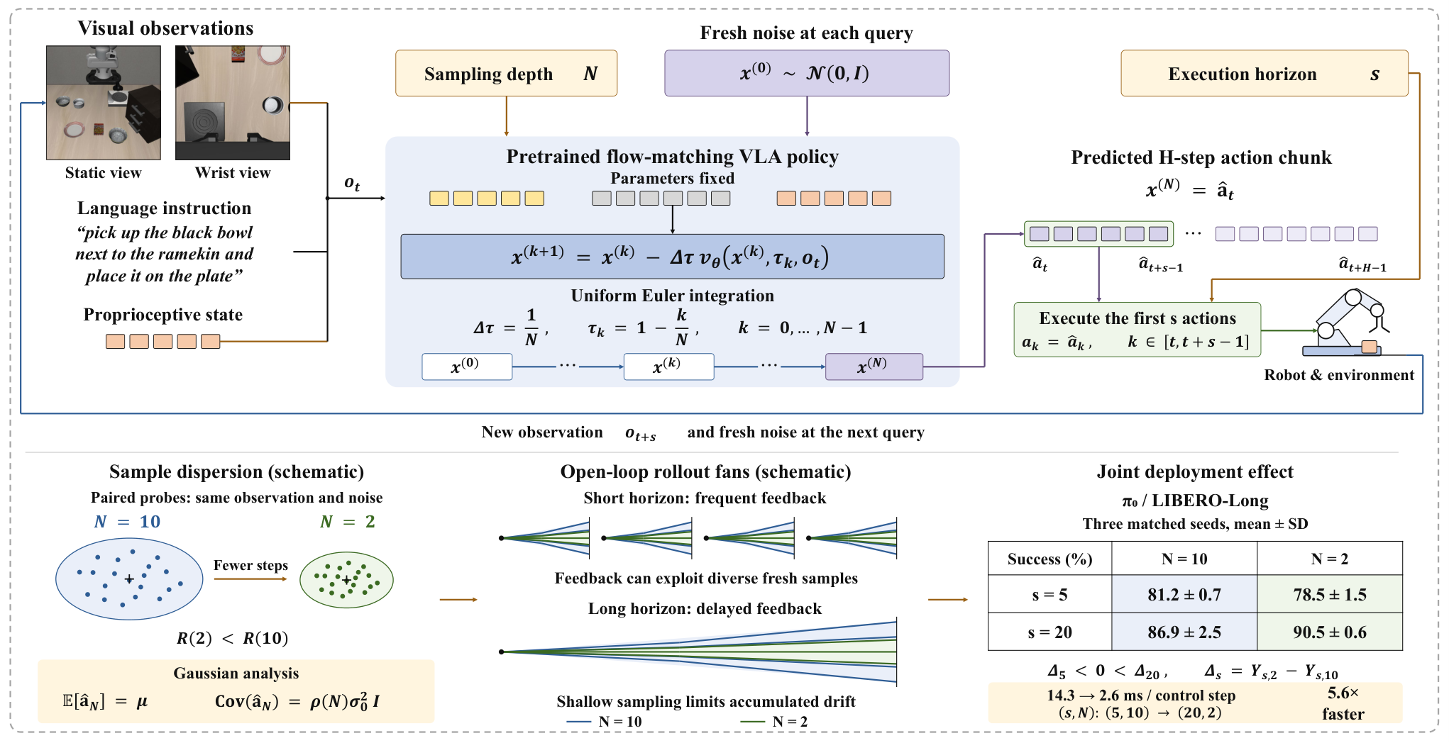
One control cycle, in order:
- Read the observation: camera images, joint state and the language instruction.
- Draw fresh Gaussian noise as the starting point of the action sequence.
- Integrate for steps to turn the noise into an action chunk of length .
- Execute the first actions without new observations.
- Go back to step 1.
The paper's contribution is entirely about how steps 3 and 4 interact. Model weights do not change; only two integers used at deployment do.
Why do fewer steps make actions tighter?
Integration uses the simplest forward Euler method, moving a small distance along the current predicted velocity at each step:
Here is the intermediate action sequence at step , is the velocity predicted by the VLA, is the flow time (from 1, pure noise, to 0, the final action), and is the current observation. Fewer steps means bigger jumps.
In a simplified case that can be solved exactly, the authors prove the following. If true actions are Gaussian with mean and variance , the mean of the generated actions is exactly for any number of steps. Only the variance changes: steps give variance , where rises from 0 toward 1 as grows. In other words, fewer steps do not bias the trajectory; they only narrow the spread around the mean trajectory. With the spread collapses to zero; as goes to infinity it recovers the true width.
Why does the mean stay put? On the mean trajectory the velocity field is constant, and Euler integration is exact for constant velocity, so one step and ten steps land at the same point. The deviation from the mean is multiplied by a factor at every step. The first factor is : 0.5 for , which halves the deviation at once, and 0.9 for , which removes only a tenth. Near the end of the flow the factor exceeds 1 and the deviation spreads out again. With many steps the integration runs the full contract-then-expand cycle and recovers the true width; with few steps the large first contraction dominates and the expansion stays incomplete, so the final spread is narrower.
A hand calculation (illustrative): suppose the true spread radius is 2 cm. The paper measures the radius at about half of the radius, so ten-step sampling gives about 2 cm of lateral deviation and two-step sampling about 1 cm. If deviation keeps accumulating in roughly the same direction during blind execution, after 20 steps the lateral drift of the two settings also differs by about a factor of two.
Why does the same change flip sign?
A narrower spread is neither good nor bad by itself; it depends on the horizon.
At short horizons the robot redraws noise and replans every few steps. With ten-step sampling each new trajectory differs more, and that diversity combined with frequent visual feedback amounts to trying different corrections, which helps the robot escape stuck states. With two-step sampling all trajectories crowd around the mean, fewer corrections are tried, and success drops slightly.
At long horizons the robot follows one sample for many steps. A wide spread is now harmful: the off-mean part accumulates into drift during blind execution. Two-step sampling narrows the spread, acting like a low-pass filter on the actions, so blind execution is more stable.
Think of walking with your eyes closed and opening them every steps. The interval between looks is the horizon ; how random your heading is at each start is the spread set by . If you look often, a slightly varied heading helps you find a way around obstacles. If you look rarely, a small heading error ends far off course, so a steadier heading is better.
Experiments: how general is the effect?
The authors want to show three things: the effect holds across models and benchmarks; the mechanism really is spread contraction; and it holds on real hardware.
The main simulation results use four LIBERO subsets (500 trials each) and 50 bimanual tasks in RoboTwin 2.0 (100 trials each), with official released weights for three open VLA backbones and no retraining.
| Model | Short horizon + default steps | Short + 2 steps | Long horizon + default steps | Long + 2 steps | Latency per control step |
|---|---|---|---|---|---|
| (LIBERO, 4-subset mean) | 92.4% | 92.0% | 92.9% | 95.5% | 14.3 ms → 2.6 ms |
| (LIBERO, 4-subset mean) | 96.9% | 97.0% | 97.6% | 98.0% | 14.2 ms → 5.1 ms |
| GR00T-N1.7 (LIBERO, 4-subset mean) | 93.2% | 91.7% | 95.7% | 95.1% | 55.6 ms → 9.9 ms |
The last column is inference latency amortized per control step; the left side of the arrow is short horizon with default steps, the right side is long horizon with 2 steps, so it reflects changing both knobs. Short and long horizons are 5 and 20 for , 5 and 10 for , and 2 and 8 for GR00T, whose default is 4 integration steps. The sign reversal is clearest on : the interaction effect (the gain from fewer steps at the long horizon minus the gain at the short horizon) is +6.4 points on LIBERO-Long. For models like with 50-step chunks, the best number of steps clearly gets smaller as the horizon grows. is already near 98%, leaving little room, and the authors mark those cells as ceiling-limited. For GR00T at the long horizon, 4 steps are slightly better than 2, so its best point sits near the released default.
RoboTwin 2.0 is a bimanual manipulation simulation benchmark; both models here use versions fine-tuned to output 50-step chunks. When replans every 10 steps, cutting integration to 2 steps lowers mean success from 73.8% to 66.9%, with 36 of 50 tasks getting worse. At a horizon of 25 the loss mostly disappears (71.7% with 10 steps, 70.8% with 2), which means the penalty for shallow sampling is tied to short horizons.
Moving from the default of replanning every 10 steps with 10 integration steps to replanning every 25 steps with 2 integration steps takes from 73.8% to 70.8% while amortized latency per control step falls to about 1/3.5; the same switch takes from 37.0% to 45.7%. This means that on bimanual tasks, long horizons with shallow sampling buy a large latency cut for a small success cost.
The mechanism is checked in two ways. The first measures action geometry directly. For the same image and the same batch of initial noise, the spread radius with is 0.51 of that with . The spread radius is the mean distance from each sample's action sequence to the batch mean. The two batch means differ by 0.208, only 3.2% of the typical action magnitude: the center barely moves and mainly the spread shrinks, although the authors find the shape of the spread changes too rather than shrinking uniformly, and simply scaling down the initial noise does not reproduce the benefit. LIBERO actions are relative end-effector displacements, so the authors add up each sample's first actions to get the path the end effector travels during blind execution, and measure how widely those paths fan out perpendicular to the direction of travel. With that width is 2.1 times the width, close to the 2.0 predicted from the single-sample spread. The simplified theory holds roughly on real billion-parameter models.
The second is causal interventions (, LIBERO-Long, mean of three seeds):
| Condition | , | , | , | , |
|---|---|---|---|---|
| Default sampling | 81.2% | 78.5% | 86.9% | 90.5% |
| Same noise at every replan | 42.3% | 72.9% | 75.0% | 89.3% |
Row two asks whether the advantage of deep sampling at short horizons comes from the diversity of redrawing noise. With noise frozen, at the short horizon collapses from 81.2% to 42.3%, while drops only 5.6 points. Deep sampling really does rely on fresh noise when replanning often.
The authors also swapped solvers. Euler evaluates the velocity once at the current point per step. Midpoint takes half a step, evaluates the velocity there, and uses it for a full step. Heun takes a full step, evaluates the velocity at the predicted end point, and averages the two velocities. With the same budget of two network calls at , Euler (two steps) reaches 90.5%, midpoint (one step) 72.5%, and Heun (one step) only 4.4%. The authors' explanation: multi-stage methods query the network at extrapolated points far from the training data, amplifying error. Teams tempted by higher-order solvers should take note.
On hardware, a 7-DoF Franka arm ran 5 tasks with 50 teleoperated demonstrations each; each backbone was fine-tuned, and each configuration got 40 trials, 2,400 in total.
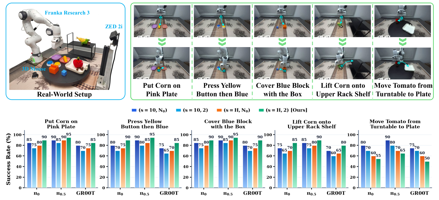
On the four static tasks, full-chunk blind execution with 2 integration steps improves success by 10.0 points for , 6.9 for and 11.3 for GR00T. With and , needs only 0.04 network calls per control step on average (the default is 1). The effect is not a simulation artifact; it holds on real hardware.
Limitations I see
First, dynamic tasks fail outright. With a turntable spinning at 5 RPM, long horizons fail no matter how many steps are used. The recipe fits tasks with essentially static objects; tracking moving objects or reacting to obstacles in real time needs short horizons.
Second, fine insertion is out of scope. The authors note that peg insertion with millimeter clearance or pressing small switches lets small angular errors accumulate beyond tolerance during long blind execution, so short horizons with deep sampling are needed. Real tasks often mix coarse transport and fine contact, so one fixed is not enough and the setting must switch by phase, and teams have to decide when to switch for their own tasks.
Third, the gain depends strongly on chunk length. The released used on LIBERO outputs only 10 actions per chunk, capping the horizon at 10 (RoboTwin uses a version fine-tuned for 50-step chunks), and the LIBERO mean improves by only a few tenths of a point; GR00T at long horizons is slightly worse with 2 steps than with its default 4. Models with short chunks may gain little.
How a robot learning team could try it
- Sweep a small grid on your own simulation evaluation: at the default, half a chunk and a full chunk; at 2 and the default. Four to six cells show whether your model has the sign reversal.
- If it does, pick a long-horizon, shallow-sampling point and record both success and average latency per control step, to confirm compute is saved without losing success.
- Split by task phase: use long horizons and shallow sampling for coarse motions such as transport and approach, and switch back to short horizons and default steps for contact, insertion or moving targets.
- Before moving to hardware, confirm the solver is forward Euler. If you use midpoint or Heun, switch back to Euler before compressing steps.
Verdict
The key lesson: sampling depth is not only a precision-latency trade-off; it also controls how spread out the actions are, and whether spread helps depends on how long the robot runs blind. When tuning VLA deployment, sweep and together.
| Aspect | Assessment |
|---|---|
| Importance | High. VLA inference latency is a main bottleneck for real deployment, and nearly every team tunes these two parameters |
| Novelty | Medium. No new model; the contribution is finding the coupling and giving a testable geometric explanation |
| Evidence | High. Three backbones, two simulation benchmarks, 2,400 real-robot trials, plus causal interventions and a solver comparison |
| Engineering cost | Very low. No training, no architecture change, only two deployment parameters |
| Worth trying | Yes, for teams running flow-matching VLAs on static manipulation tasks, who can try it the same day; do not copy it to dynamic or fine-insertion tasks |
How did this read for you?
Hoot made a note. Thanks for the feedback.

One tap, no sign-in; tap again to undo. Only anonymous counts are kept, never who you are.
Discussion
Add experiment details, reproduction notes or a different take. Requires a GitHub sign-in.
Loading the discussion…