Contents · 8 sections
1What problem is it really solving?2How HERO works: the overall picture3Why two teachers, and how are examples assigned?4Why add the true paths of unpopular items?5Experiments: more accurate, and more balanced?6Where I think it falls short7How a recommendation team could try it8VerdictSHARE

Teams that run generative recommendation and are considering distillation for post-training should read this, because it exposes a side effect that overall metrics hide. On-policy distillation (OPD), where the student generates on its own and a teacher gives a full probability distribution at each position, makes generative recommenders train faster, but the student drifts further and further toward popular items. The bias comes from two places: the teacher's probabilities already favor the SIDs of popular items, and the student rarely generates the SIDs of unpopular items, so those paths get almost no supervision. The paper's method, HERO (an on-policy distillation framework with two specialized teachers plus extra supervision on unpopular paths), handles the two sources separately. It trains a popular-item teacher and an unpopular-item teacher. Each training example goes to the teacher that matches the group of the item the user actually clicked, and the true SIDs of unpopular items are also sent to the unpopular-item teacher. Only the student is served.
In a 15-day A/B test on the "Guess What You Like" module of the 1688 homepage, GMV rose 3.412% over the existing generative recommender. Offline on 1688 data, the hit rate on unpopular items rose from 0.5301 with standard OPD to 0.5416. How far the ratio "share of exposure over share of demand" for the popular and unpopular groups sits from 1 fell from 0.715 to 0.392; smaller means exposure tracks users' real demand more closely. Distillation passes on more than knowledge: it also passes on the teacher's taste for popular items.
What problem is it really solving?
In generative recommendation the model reads the user history and generates the SID of the next item one position at a time. Plain SFT learns only the single token of the true item at each position. OPD supervises differently: the student first generates SIDs itself, then on every prefix the student visited, the teacher gives a probability for every candidate next token, and the student matches that whole distribution. Tokens that were never clicked also get a signal, so supervision is denser. In the paper's Figure 1a, OPD uses about 5% of the training budget to beat the click hit rate that SFT reaches with the full budget.
The trouble is that bias gets amplified. Picture an e-commerce homepage (illustrative): a user just bought storage boxes, and the item they actually click is a folding shelf that sells poorly.
| Item (illustrative) | Popular or unpopular | Teacher's probability for the first token | Reached by the student's beam search? |
|---|---|---|---|
| Best-selling storage bin | Popular | 0.50 | Yes |
| Best-selling hanger | Popular | 0.30 | Yes |
| Folding shelf (true click) | Unpopular | 0.05 | No |
After matching the teacher, the student pushes the popular items' probabilities up a little more. In the next round of generation it reaches the shelf's path even less often, so that path receives even less teacher supervision. The two effects feed each other, and the bias grows round after round.
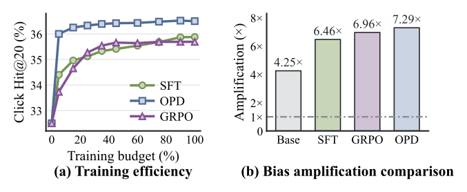
The paper measures this with an amplification ratio: the share of popular items among the model's generations divided by their share in the candidate set. Among the values marked in Figure 1b, SFT reaches 6.46x and OPD 7.29x, which means OPD makes the student lean toward popular items more than SFT does. Popular and unpopular are split by interaction counts in the training period: on 1688, an item with at least 4,096 interactions counts as popular, and everything else as unpopular.
How HERO works: the overall picture
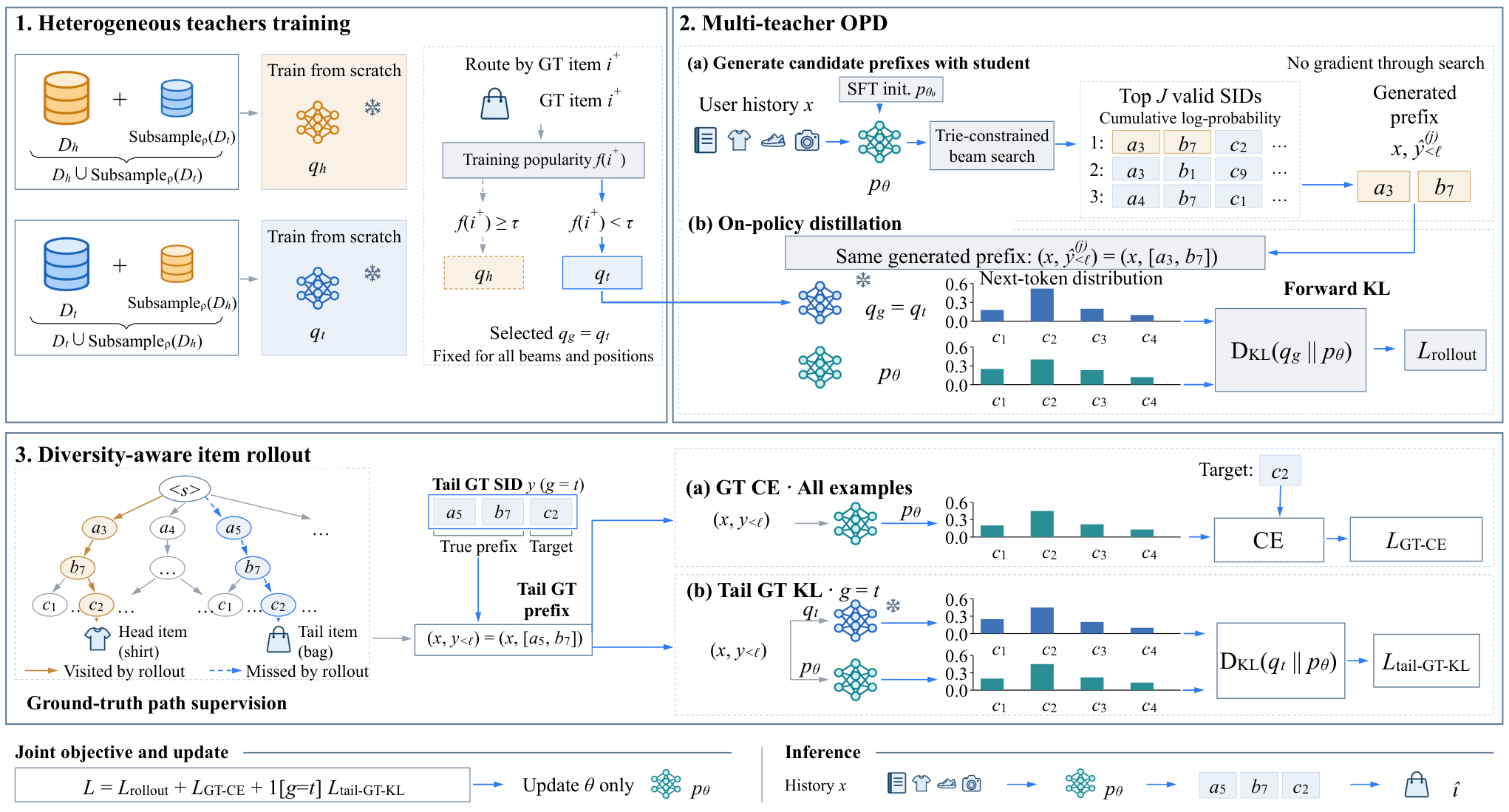
Training has three steps, and in the end only one student model is served:
- Train the two teachers offline. The popular-item teacher uses all popular-item examples plus a random 10% of the unpopular-item examples; the unpopular-item teacher does the reverse. Both teachers have exactly the same architecture as the student. The teachers are each trained from scratch and stay frozen during distillation; the student starts from the SFT model and is the only model updated during distillation.
- The student generates and the teacher scores. Each example picks its teacher by the popularity of its true item. The student runs beam search to produce 32 SIDs, and on every prefix of each one it is matched to the chosen teacher's next-token distribution.
- Add supervision from the true SID. Every example gets cross-entropy on its true SID; when the true item is unpopular, the unpopular-item teacher also supervises the student along the prefixes of the true SID.
The key division of labor: the choice of teacher decides whether the signal is biased, and the added true paths decide whether unpopular items get a signal at all. The parts are taken one at a time below.
Why two teachers, and how are examples assigned?
With a single teacher, every example receives a distribution that favors popular tokens. HERO replaces it with two specialized teachers. They are not larger models; they are the same size and differ only in the mix of training data. The unpopular-item teacher has seen mostly unpopular items, so its probabilities on their SIDs are more accurate.
The assignment rule looks at the item this example's user actually clicked. If the true item is popular, the example goes to the popular-item teacher; if it is unpopular, to the unpopular-item teacher. Training and inference must be kept apart here: the true item exists only in the training data, so assignment happens only during training. At inference neither teacher takes part, and the student generates SIDs directly from the user history without knowing whether the target is popular.
How are student and teacher matched? Given a user history, the student uses beam search to generate 32 complete SIDs. The search may only reach items that actually exist; the paper restricts the tokens allowed at each step with a prefix tree. For every position of every SID, the part generated so far is fed as a prefix to both the student and the chosen teacher, each outputs a full distribution over the next token, and forward KL pulls the student toward the teacher:
Here is the user history, is the first tokens of the student's -th generation, is the teacher chosen by the true item's popularity, is the student, and . The student supplies the prefixes and the teacher supplies the learning signal; gradients do not flow through beam search, and only the student's outputs on those prefixes are updated. Hoot says

- The prefix tree governs the search: it only makes every beam path a real item; the learning signal is the teacher's distribution on those prefixes.
- The true item only picks the teacher: it never enters the student's input, so nothing is missing at inference.
Illustrative example whose true click is an unpopular item. The left column exists only during training; bottom right is inference, where neither the teachers nor the true item are present. Source: paper §3 (two teachers assigned by the true item's popularity, beam width J=32, prefix-tree-constrained search, forward KL updates only the student)
Why not simply average the two teachers' distributions half and half? The ablation includes exactly that: on 1688, a fixed half-and-half mix gives an unpopular-item hit rate of 0.5252, while assigning by the true item gives 0.5416. This shows the teacher has to match the example. As for why the half-and-half mix does worse, my guess is that the mixed distribution still leans toward popular items.
Why add the true paths of unpopular items?
Changing teachers only fixes whether the signal is biased. A path the student never generates cannot be supervised, however accurate the teacher. HERO's second design fills in those paths.
The example in the paper's Figure 2: an example's true item is an unpopular bag, whose SID in the figure is [a5, b7, c2]. The student's beam search goes through [a3, b7] and never reaches a path starting with a5. Because this example was already assigned to the unpopular-item teacher by its true item, that teacher supervises two prefixes: [a3, b7], which the student visited, and the true [a5, b7]. The supervision on the true prefix [a5, b7] is the new term, with the same formula as above but the prefix taken from the true SID:
is the first tokens of the true SID and is the unpopular-item teacher. This term is computed only for examples whose true item is unpopular. Every example also keeps ordinary cross-entropy on its true SID. The total objective adds the three terms with weight 1 each and updates only the student.
This is different from up-weighting unpopular examples. Up-weighting only makes the loss on the single true token larger; here the unpopular-item teacher gives a whole next-token distribution on the true prefix, so the other candidate tokens under that prefix get a signal too. The paper tests up-weighting directly: in the continued-SFT setting (SFT++), raising the cross-entropy weight of unpopular examples from 0.5 to 8 never catches HERO on either overall or unpopular-item hit rate (Figure 3).
Experiments: more accurate, and more balanced?
The offline experiments use 1688 data and three public datasets (Amazon Beauty and Pet, and MovieLens-1M). On 1688 the metrics check whether the top 240 recommendations hit a click, a payment, or a click on an unpopular item; on the public data they use the top 20.
Balance is measured two ways. The first is DTR (demand-to-recommendation ratio), which compares exposure with demand: the popular items' share of exposure (with higher-ranked slots weighted more) divided by their share of demand, divided again by the same ratio for unpopular items. A value of 1 means exposure is proportional to demand. An illustrative case: popular items make up 50% of clicked demand but 75% of exposure, a ratio of 1.5; unpopular items make up 50% of demand and 25% of exposure, a ratio of 0.5; DTR is then 3, heavily tilted toward popular items. The table reports how far DTR is from 1, so smaller is better. The second is ORR (output concentration), the share of all recommendation slots taken by the 5 most frequently generated items; smaller means less piling onto a few items.
| Method (1688) | Click hit | Pay hit | Unpopular-item click hit | Distance of DTR from 1 | ORR |
|---|---|---|---|---|---|
| SFT | 0.5742 | 0.7562 | 0.5302 | 0.654 | 0.0027 |
| Standard OPD (GKD) | 0.5786 | 0.7584 | 0.5301 | 0.715 | 0.0029 |
| BEAR | 0.5763 | 0.7571 | 0.5351 | 0.479 | 0.0028 |
| HERO | 0.5819 | 0.7607 | 0.5416 | 0.392 | 0.0025 |
Standard OPD in the table is the baseline GKD (a single teacher trained on all the data distils along the student's generated paths, and cross-entropy on the true SID is kept). It lifts click hit a little, leaves unpopular-item hit unchanged, and pushes DTR further from 1. That is the opening point in action: overall metrics alone do not show that distillation made recommendations more skewed. HERO is highest on all three hit metrics and has the DTR closest to 1, which shows accuracy and balance can be gained together. Across all four datasets HERO has the best overall and unpopular-item hit rates. On MovieLens-1M, the baseline BEAR (a search-aware training method for generative recommendation) has a lower ORR (0.0418 against 0.0434), but its overall hit rate of 0.1896 is below HERO's 0.1936, which shows that less concentrated output does not by itself mean better recommendations.
The 1688 ablation separates the roles of the parts fairly cleanly. Sending every example to the popular-item teacher (this variant also drops the unpopular true-path term) raises the distance of DTR from 1 to 2.736 and drops unpopular-item hit to 0.4977; sending every example to the unpopular-item teacher drops click hit to 0.5463. This shows a single teacher always sacrifices one side. Removing the KL on the student's generated paths drops unpopular-item hit to 0.5222, the largest fall among the three loss terms; removing the unpopular true-path term lowers unpopular-item hit from 0.5416 to 0.5329 and raises the distance of DTR from 1 from 0.392 to 0.742, which shows the term affects both unpopular-item hit and exposure balance.
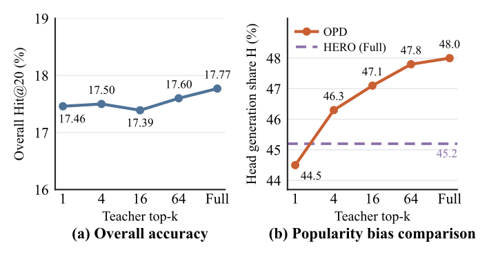
One more experiment tests "denser means more skewed" directly. On MovieLens-1M, only the teacher's k most probable tokens are passed to the student. As k goes from 1 to the full vocabulary, overall hit moves only between 17.39% and 17.77%, while the share of popular items among generations rises from 44.5% to 48.0%. HERO with the full distribution sits at 45.2%, which shows it keeps the full distribution while holding back this shift. These readings come from Figure 5. The authors take this to mean that the teacher's lower-ranked tokens also carry a popularity preference, so denser supervision may pass on more of it.
The online A/B ran from 24 September to 9 October 2026, with users randomly split into groups of equal traffic. Against the existing generative recommender, GMV rose 3.412% (95% confidence interval 0.759% to 6.065%). Because only the student is served, response time did not change noticeably, which means the gain was not bought with extra inference cost. Per-user exposure, per-user clicks and click-through rate on unpopular items also improved.
Where I think it falls short
First, the online gain has a wide interval. The 95% confidence interval for the GMV lift runs from 0.759% to 6.065%, with a lower bound under 1%. The offline absolute gaps are small too: click hit on 1688 goes from 0.5786 with standard OPD to 0.5819. So I would treat 3.412% as a credible direction whose size still needs to be reproduced.
Second, training cost rises noticeably. The student starts from the SFT model, and distillation is a fairly short post-training stage (on 1688 it uses only the last four days of the training window). But besides the student, two teachers of the same size must be trained from scratch, and during distillation every example runs a width-32 beam search and then a teacher forward pass on every prefix. Inference costs nothing extra, but the offline compute should be budgeted up front.
Third, popular and unpopular are a single hard split into two groups. On 1688 the line is 4,096 interactions, so an item just over the line and one far above it share a teacher. On the public data the unpopular-item hit rate only counts unpopular items that appear in training; items never seen in training are left out, so how much it helps cold-start items cannot yet be seen.
How a recommendation team could try it
- Measure the bias first. On an existing distilled or post-trained model, split items into popular and unpopular by interaction count and compute the amplification ratio and DTR. Only if DTR clearly worsens after distillation is it worth going further.
- Next, run OPD with teachers assigned by the true item, without the unpopular true-path term yet. Use the existing single-teacher OPD and a "half of each teacher" mix as controls, to confirm the gain comes from matching examples to teachers rather than from simply having an extra teacher. Check whether unpopular-item hit and DTR improve while overall hit holds.
- If that works, add the unpopular true-path term. Do not skip distillation on the student's generated paths and distil only along true paths: the paper's baseline that does this, GT-KD (distillation only along true SID prefixes), has a distance of DTR from 1 of 0.994 on 1688, worse than SFT's 0.654.
- Online, watch per-user exposure and click-through rate on unpopular items, and the share of slots taken by the top 5 items, alongside GMV, to confirm the gain was not bought with more concentrated popular recommendations.
Verdict
When generative recommendation uses distillation for post-training, look beyond overall hit rate and check whether the teacher has skewed the popularity mix of recommendations; HERO's answer is to match teachers with different preferences to the right examples and to add supervision on the unpopular paths the student never reaches.
| Dimension | Assessment |
|---|---|
| Importance of the problem | High. OPD is being adopted for post-training generative recommenders, and the popularity bias it brings cannot be seen in overall hit rate |
| Novelty of the method | Medium-high. Two teachers and assignment by target are not complex, but treating the two sources of bias, the teacher and the student's own generation, separately is a clear idea |
| Strength of evidence | Fairly strong. Four datasets, a full ablation, a density experiment and a 15-day online A/B, though the confidence interval on the online lift is wide |
| Engineering cost | Medium-high. Two extra teachers to train and 32 beams per example during training; inference unchanged |
| Worth trying? | Yes. Generative recommendation teams that already use distillation and care about long-tail exposure can start with assigning teachers by the true item, then add the unpopular true-path term |
How did this read for you?
Hoot made a note. Thanks for the feedback.

One tap, no sign-in; tap again to undo. Only anonymous counts are kept, never who you are.
Discussion
Add experiment details, reproduction notes or a different take. Requires a GitHub sign-in.
Loading the discussion…