Contents · 7 sections
1A few terms used later2Why pull relevance on the sparse codes3Walkthrough: which side the four most distinctive neurons favor4In-domain gains, and what happens on a new corpus5Do these neuron meanings still hold on a new corpus6What this means for people who build medical retrieval7LimitationsSHARE

The passage with the answer sat at rank 23: how a sparse autoencoder unpacks this medical retrievalSomeone asks: "What lab monitoring should be done in neonatal patients on oral retinoids, and at what frequency?" Retrieval has to find the passages that can answer that question among about 244,000 medical passages.
The passage at rank 4 discusses isotretinoin laboratory abnormalities. It is about acne patients and never mentions children or neonates. The passage that actually writes the answer says serum lipids and liver function tests should be checked at baseline, one month after starting treatment, and every three months thereafter. It sits at rank 23.
All you see is a similarity score between two vectors and a list of ranks. You cannot see which senses the system is actually comparing.
This paper is from Doctolib AI Research Lab in Paris. It aims to give medical retrieval an explanation that a person can read, and that can transfer to a new corpus. The usual approach is a general-purpose text embedder such as BGE, or MedEmbed, which is BGE fine-tuned on clinical data: queries and documents become dense embeddings and are ranked by cosine similarity. The dimensions are entangled, so it is hard to say which senses pushed a document up the list. Sparse autoencoders (SAEs) have mostly been used on internal activations of large models, to split entangled features into a higher-dimensional space where only a few fire at a time. Kang et al. applied them to BGE embeddings on the general retrieval set MSMARCO, and used a KL divergence to stay aligned with the relevance structure the original model had already learned. The authors do not carry that assumption over to medical corpora, because the training data for bge-large-en-v1.5 and gemini-embedding-001 are not public. So they freeze the embedder and train a TopK SAE on its dense embeddings: a reconstruction loss keeps information from the original vectors, and an InfoNCE term that uses ground-truth query-document labels pulls the sparse codes of relevant pairs closer. On the clinical retrieval benchmark CURE, original BGE NDCG@10 is 53.06, and the same contrastive training at full original width (k=1024) reaches 61.87; keeping only 128 or 256 active dimensions still reaches at least 94% of that dense score. On five unseen medical retrieval sets, the sparse models lose less than their dense contrastive counterparts, especially when the target corpus is farther from CURE. Feature interpretations written only on CURE still give a positive signal for predicting whether a neuron will fire on these new corpora.
Sparse features can unpack a single retrieval, and the interpretations can transfer to a corpus the model never saw; but models trained on CURE still fall below the original embeddings on most out-of-domain sets.
A few terms used later
A dense embedding is a length-d vector of real numbers: 1024 dimensions for BGE and MedEmbed, 3072 for Gemini. An SAE first maps it into a wider space of width m, for example 3072, then keeps only the k largest activations and sets the rest to zero. The paper calls this a TopK SAE, following Gao et al. (2024). What you get is a sparse code: most positions are 0, and the ones that fire are often easier to read as a sense, such as infant health, without a guarantee that every position maps to a single clear concept.
Retrieval compares the cosine similarity of the query and document sparse codes. During training the embedder stays frozen; only the SAE is updated.
The paper also calls a model dense when k equals the original embedding dimension and the hidden width is still expanded to some m larger than d. The hidden layer is still wider than the original dimension, TopK keeps at most d non-zeros, and contrastive training is still on, but the number of active units is capped at the original width. Later we call this baseline the dense model. The 61.87 figure is BGE at k=1024, not the much sparser k=64 code. Ranking quality is NDCG@10, which looks at the first ten results and rewards relevant documents that appear higher; the paper reports it in percent.
CURE is the clinical retrieval set used for training: about 244,600 passages and 2,000 questions, split 1,400 / 200 / 400 for train, validation, and test, drawn mainly from academic biomedical literature. Five other sets are used only for evaluation and are never trained on. MIRIAD (a biomedical literature retrieval set) and NFCorpus (a medical nutrition retrieval set) are closer to CURE in genre. R2MED (a medical community Q&A retrieval set) has three subsets (Biology, Bioinformatics, Medical-Sciences) whose queries come from StackExchange and whose corpus is more Wikipedia-like, so they sit farther from CURE.
Why pull relevance on the sparse codes
If you only reconstruct the dense embeddings, the sparse codes still hold information from the original vectors, but that does not guarantee that a query and its relevant documents are pulled closer. Prior work on MSMARCO used a KL divergence to stay aligned with the relevance already encoded by the original BGE model. Here the corpus is medical and the original models' training data are not public, so the authors switch to labeled InfoNCE: each query is paired with one document already marked relevant, and the two sparse codes are pulled together. Negatives come from the other paired documents in the same batch, plus the document batch used for reconstruction; other known relevant documents among those candidates are masked out of the denominator. The total loss is the reconstruction term plus λ times InfoNCE.
Setting λ to 0 turns the contrastive term off and leaves only reconstruction. On CURE that term matters. For a baseline with both k and m equal to the original dimension and no expansion, reconstruction-only BGE NDCG@10 is 7.5 points below the contrastive version, and no higher than the original embeddings. The sweep plots later show the same pattern: the gray line (λ=0) sits on or below the dashed original-BGE line, and in-domain scores rise clearly only after InfoNCE is added.
Walkthrough: which side the four most distinctive neurons favor
The example below is the neonatal retinoid query from the paper's Figure 1. All numbers come from the paper. The model is an SAE trained on BGE embeddings, with 64 neurons active at a time and total width m=3072. The authors pick the four neurons whose activations differ most between the query's two passages. The numbers are ℓ2-normalized activations on each text. Rankings are cosine similarity of the sparse codes over all 244,600 CURE passages.
Step 1. Look at what the query itself fires. The four neurons are named laboratory, retinoids, surveillance, and infant health, with activations 0.183, 0.400, 0.220, and 0.400. The question involves both the drug and the labs, and the neonatal population; retinoids and infant health are equally strong at 0.400.
Step 2. Look at passage A, ranked 4 and labeled not relevant. It discusses isotretinoin laboratory monitoring in acne patients and never mentions children or neonates. The four activations are 0.306, 0.375, 0.229, and 0. infant health is exactly 0. It wins on the first three lexical concepts because it repeats those words.
Step 3. Look at passage B, which writes the answer, is labeled highly relevant, and is ranked 23. It buries "serum lipids and liver function tests at baseline, after one month, and every three months thereafter" in a chunk about survival. It never writes laboratory or monitoring, so those two neurons are 0; retinoids is 0.248 and infant health is 0.109. Only the infant-health concept stands on its side.
Step 4. Ranking uses cosine similarity after ℓ2 normalization, so each dimension's contribution is the query activation times the document activation. Using the three-decimal figures in the paper, the four contributions on passage A are 0.183×0.306≈0.056, 0.400×0.375=0.150, 0.220×0.229≈0.050, and 0.400×0=0, summing to about 0.256; on passage B they are 0, 0.400×0.248=0.099, 0, and 0.400×0.109≈0.044, summing to about 0.143. Three concepts favor A, and only infant health favors B. That is why the paper's "three to one" refers to the number of concepts, not a strength ratio obtained by summing document activations. These four neurons account for 53% and 35% of the cosine similarity of passages A and B with the query.
What these numbers can show is that, among the four features that differ most and already account for more than half or about a third of the two cosines, lexical overlap favors the irrelevant passage. The full ranking still involves the remaining activations, so these four dimensions alone cannot reconstruct the complete order. They also cannot, by themselves, show that the feature names still hold on a new corpus; that is tested later with activation prediction.
In-domain gains, and what happens on a new corpus
The explanations can unpack a single retrieval. If retrieval itself is switched to sparse codes, how much of the score is left at the intermediate values of k? On the CURE test set, BGE at k=256 is 60.50±1.02 and at k=128 is 59.35±0.35, both still at least 94% of the dense 61.87, which means sparsity does not give back the in-domain gain. The dense Gemini model (k=3072) is the best in-domain result, at 62.07±0.73. For all three embedders, every k tried beats that embedder's original embeddings, and the highest score is always the dense model.
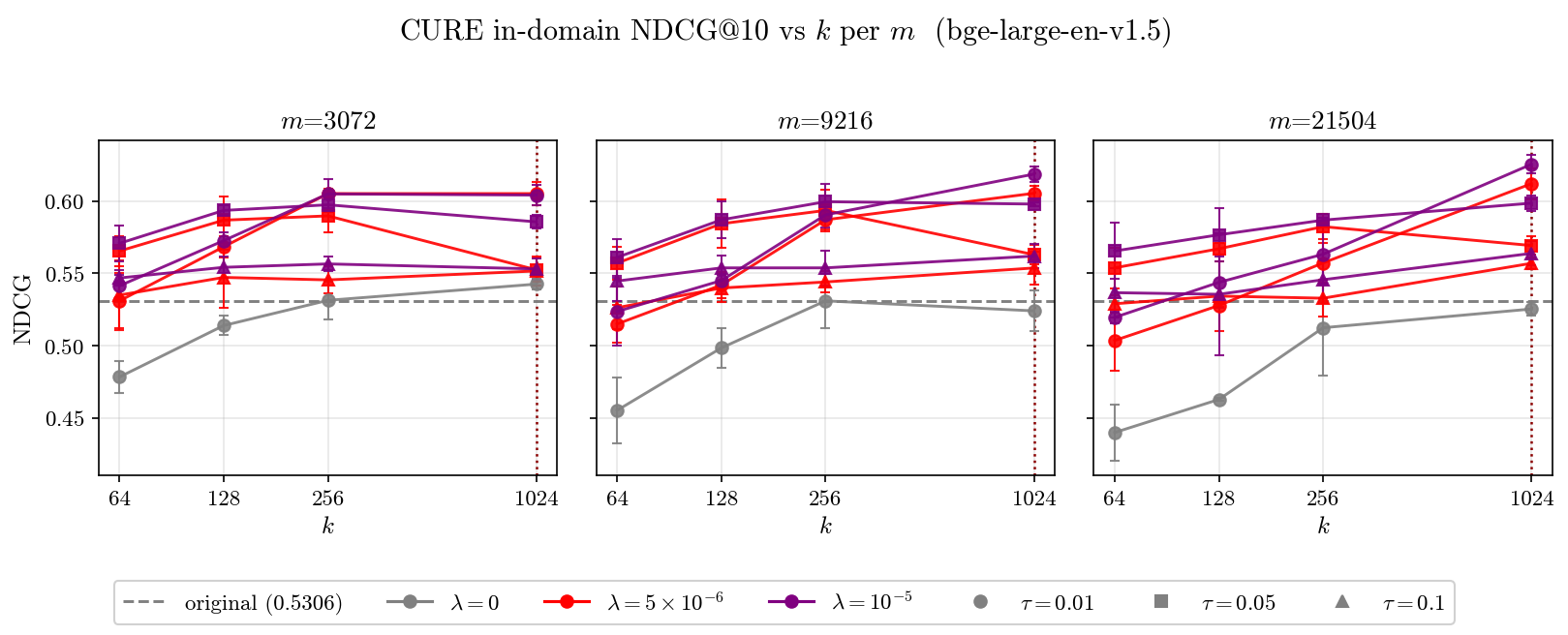
Source: paper HTML result figure, titled CURE in-domain NDCG@10 vs k per m (bge-large-en-v1.5)
Out of domain is a different story. When a model trained on CURE is applied directly to the five unseen sets, MIRIAD and NFCorpus, which are closer to CURE, improve as k grows and peak near the dense setting, but still stay below original BGE. The three more distant R2MED subsets get no extra benefit from going dense: on BGE, the k=256 means are already at least as high as dense, 28.10 vs 27.21 on Bioinformatics, 10.06 vs 8.37 on Biology, and 29.05 vs 27.33 on Medical-Sciences. That means the extra capacity does not help on the farther corpora; on Biology both are below the original 12.72, with the sparse model dropping less.
| Dataset | Original BGE | SAE k=256 | dense k=1024 |
|---|---|---|---|
| CURE (in-domain) | 53.06 | 60.50±1.02 | 61.87±0.55 |
| NFCorpus | 38.17 | 35.61±0.08 | 36.62±0.29 |
| MIRIAD | 77.24 | 73.85±0.92 | 75.05±0.36 |
| Bioinformatics | 27.04 | 28.10±0.89 | 27.21±1.98 |
| Biology | 12.72 | 10.06±1.17 | 8.37±0.65 |
| Medical-Sciences | 27.78 | 29.05±0.80 | 27.33±1.72 |
(Numbers from the retrieval results table in the paper body, NDCG@10 in percent; figures with ± are means and 95% confidence intervals over 3 random seeds)
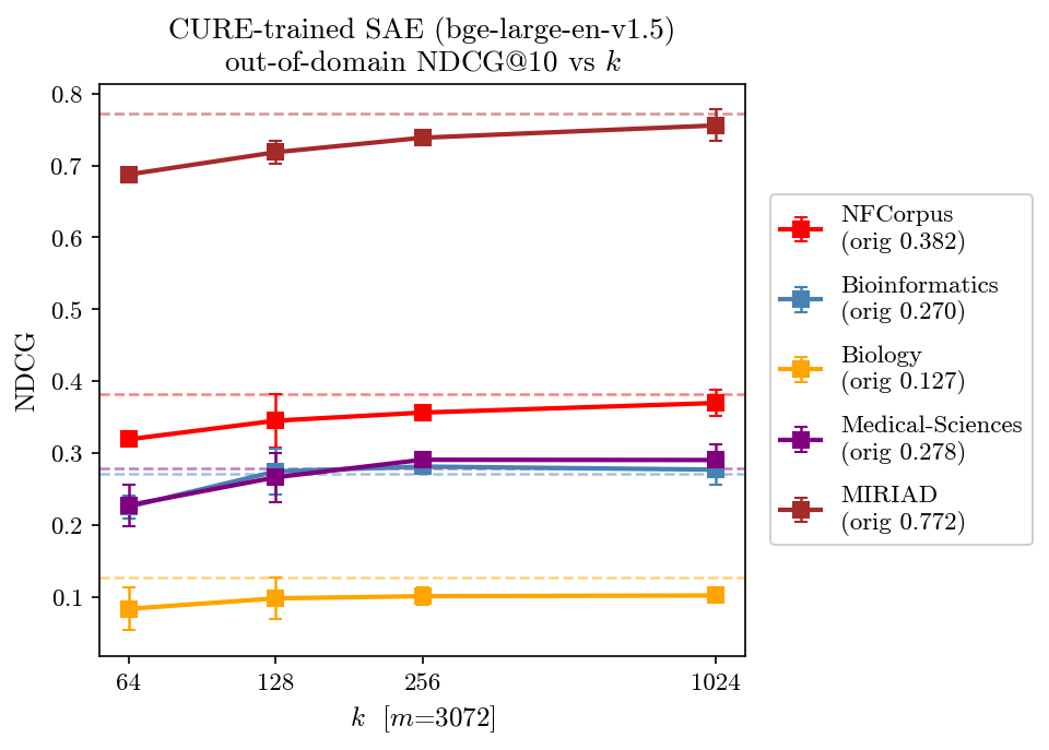
Source: paper HTML result figure, titled CURE-trained SAE (bge-large-en-v1.5) out-of-domain NDCG@10 vs k
Capacity is not only k; the total width m also matters. For dense models, in-domain NDCG@10 rises with m, while out-of-domain sets prefer a small m or do not move. When k is at most 256, the smallest m is better or tied on every set. The contrastive weight λ splits the same way: λ>0 is best in-domain; for dense models, λ=0 wins on every out-of-domain set; for sparse models (k at most 256) the gap between λ=0 and λ>0 is small, and either setting can come out slightly ahead. So when training on CURE, sparse codes lose less out of domain than dense contrastive learning.
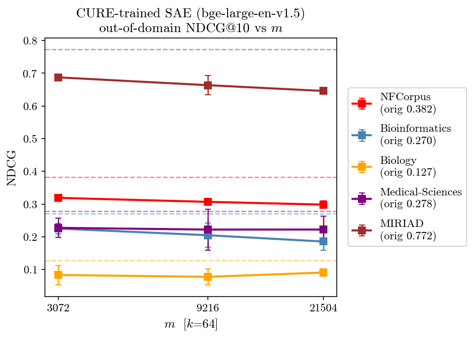
Source: paper HTML result figure, titled CURE-trained SAE (bge-large-en-v1.5) out-of-domain NDCG@10 vs m
These sweeps can show how capacity and the contrastive term twist in-domain gains together with out-of-domain drops. They cannot show whether the feature names themselves travel with the model.
Do these neuron meanings still hold on a new corpus
The feature names are built as follows. For each neuron, the authors take the 5 highest-activating documents and 5 highest-activating queries in CURE, plus 2 documents where the neuron did not fire, and produce three interpretations: the snippets themselves; the most distinctive words by TF-IDF; and an Interpreter LLM (medgemma-4b-it) that writes a short topic label, a one- or two-sentence description, and up to ten keywords. Neuron 2177, for example, is labeled bone: it reacts to text about bone tissue, bone regeneration, bone remodeling, and bone cells. Each interpretation is written once on CURE and reused as-is on the five out-of-domain sets; only the text being scored changes.
To test whether those meanings hold, the same family of model is used as an Activation Prediction LLM: given only the interpretation, it outputs the probability that the neuron will fire on a passage. If the meaning is stable, that probability should line up with a positive or negative label. A text is a positive if the neuron is among its 20 strongest active features, and a negative if the neuron is inactive. The authors measure Pearson correlation r between the predicted probability and this binary label. For the BGE SAE with k=64 and m=3072, Interpreter LLM descriptions reach r=0.440 on CURE and stay positive on all five out-of-domain sets: MIRIAD 0.334, Bioinformatics 0.290, Medical-Sciences 0.286, NFCorpus 0.257, Biology 0.226. TF-IDF is close; feeding raw snippets is worse on every set. Computed separately for each embedder and each interpretation type, activation-prediction performance correlates with retrieval NDCG@10 across the five out-of-domain sets at Pearson values between 0.69 and 0.94: the corpora on which the meanings still line up are also the ones where retrieval transfers more readily. In the same evaluation, SAE features are more interpretable than the original embeddings on every set and every description type, and also more interpretable than a contrastively trained, non-expanded baseline with k and m both equal to the original dimension. Hoot says
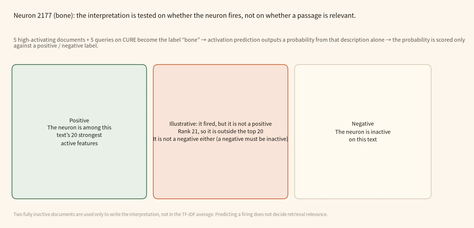
Neuron 2177 in the paper is labeled bone: it reacts to text about bone tissue, bone regeneration, bone remodeling, and bone cells. The steps below follow the same rules as the article to show how it is named and how a text is labeled positive or negative. The rank-21 boundary is illustrative, to make clear that “it fired” is not the same as “it counts as a positive.”
top 5+5 activating samples → Interpreter writes bone → activation prediction outputs a probability → scored only against a positive/negative label → outside the top 20 is not a positive
- top activating samples → Interpreter descriptionFor neuron 2177, the authors take the 5 highest-activating documents and 5 highest-activating queries in CURE to write the interpretation. Two fully inactive documents also go to the Interpreter LLM and the snippets, but they are not used in the TF-IDF average.5+5 samples used for naming; 2 inactive ones stay out of TF-IDF
- samples → the bone descriptionThe Interpreter labels this neuron bone and says it reacts to text about bone tissue, bone regeneration, bone remodeling, and bone cells. That description is written once on CURE and reused as-is on the five out-of-domain sets.write the interpretation once; only the scored text changes out of domain
- description → predicted probability → binary labelThe activation-prediction model, given only this description, outputs the probability that the neuron will fire on a new text. That probability is scored against a positive/negative label: a positive must be among the 20 strongest active features, and a negative is completely inactive.positives ⊆ top 20 active features, not every non-zero
- a rank-21 firing → not a positiveIllustrative: if a text fires this neuron at rank 21, it is neither a positive nor a negative. This test also does not say whether the text is relevant to a query.21>20, so a firing still does not count as a positive
On CURE, Interpreter descriptions reach r=0.440, and the five out-of-domain sets stay positive. These numbers measure whether a description can predict a firing; they do not replace the retrieval-ranking walkthrough in the article.
Source
Paper §6.1–6.2: Interpreter description of neuron 2177; a positive must be among the 20 strongest active features; the TF-IDF average uses only the top 5 documents and 5 queries. Rank 21 is an illustrative boundary.Five medical experts later ran a human check. The authors randomly sampled 30 neurons from the 60 with the highest interpretability scores, with 15 passages that activate and 15 that do not. Experts saw only the generated description and a text excerpt, and scored from 1 to 4 whether the neuron would fire. The average of the five experts correlated with the true labels at r=0.81, with AUROC 0.92; they classified 27 of 30 passages correctly, with 3 false negatives and no false positives. That means a clinician reading only a natural-language description can, most of the time, tell whether the feature will fire.
The paper also applies the same CURE-trained neurons to retrieval examples on Medical-Sciences and NFCorpus. In Figure 3, these neurons account for 46% and 61% of the cosine similarity in one pair of examples, and 70% and 58% in the other, ranges comparable to the in-domain examples. The ranking error in the opening of this article uses the same readable features.
What this means for people who build medical retrieval
Adding a labeled TopK SAE on top of a frozen embedder can do retrieval and explanation at the same time; when you care about transfer, look at a sparse configuration first, and do not default to running contrastive learning at the dense k=d setting.
If you already use BGE or a similar model for medical retrieval, and you need to tell a clinician or a reviewer why a passage was ranked first, you can train a k=128 or k=256 SAE on a labeled corpus. Name neurons from the queries and documents that activate them most, then, for a misranked query, spread out the features that differ most, as in the neonatal example above.
When you plan to move the model to a new specialty or genre, do not look only at in-domain NDCG. In this paper the more distant R2MED subsets did not get better by going dense, and some got worse. You can keep a smaller k and a smaller m, and use both retrieval and activation prediction on the new corpus to see whether the feature meanings are still there.
Limitations
The human check covered only 30 neurons and five clinicians, so the study remains small.
Interpretability scores rely mainly on a large language model. The authors also reran the evaluation with Qwen2.5-3B-Instruct and Gemma3-4B, and the correlations stayed positive, but calibration remains an issue.
Sparse codes do not match dense retrieval on every set.
How did this read for you?
Hoot made a note. Thanks for the feedback.

One tap, no sign-in; tap again to undo. Only anonymous counts are kept, never who you are.
Discussion
Add experiment details, reproduction notes or a different take. Requires a GitHub sign-in.
Loading the discussion…