SHARE

With AI-generated content, an advertiser can make many different cover images and titles for the same game at almost no cost, but each creative gets very few impressions, and the system has a few milliseconds to decide which ones go to the ranker. This Roblox paper adds a creative pre-ranking layer between recall and ad ranking: when a new creative lacks data, it first borrows the history of its campaign, its game and its target audience, then draws one random score from the uncertainty of that estimate, so untried creatives still get a chance to be shown. On replayed live traffic, its shortlist lifts the ranker's predicted play-through rate by 8.14%, against 2.80% for a random shortlist of the same size, while the whole pipeline gets only 0.2% slower. After an A/B test it now serves production.
Teams working on ads or content recommendation should read it, because it addresses a common stage that is rarely modeled with care: before the ranker, each campaign has several creatives and only one or two can be sent on, and which ones are sent decides which ones ever collect data. The method is almost entirely closed-form statistics with no hyperparameters to tune, and online it does one weighted sum and one Beta draw, so it is easy to copy. One caveat: the main evidence is a frozen offline replay that scores shortlists with the ranker's predicted play-through rate rather than real plays, so the long-term value of exploration does not show up in it.
What problem is it actually solving?
Below is one ad creative for a game; the same game carries several such images with different titles.

Take an example (illustrative). A shooter game runs a campaign with 3 creatives:
| Creative | Past impressions | Past plays | Raw play rate |
|---|---|---|---|
| A: old cover | 20,000 | 400 | 2.0% |
| B: made last week | 50 | 2 | 4.0% |
| C: uploaded today | 0 | 0 | none |
Ranking by raw rate puts B first, but 2 plays out of 50 impressions may be luck; C has no data and cannot be ranked at all. Ranking by a point-estimate CTR model, A has the most data and the most stable estimate, so A is likely sent to the ranker every time. B and C never collect data, and the model never learns whether they are better.
The paper places this problem at a specific point: after recall, before ranking. The ranker is a heavy per-user model whose cost grows with every extra candidate, so not every creative can be sent. In the replay, a request recalls just under 500 campaigns and more than 1,000 creatives, about 2.6 per campaign. Sending all of them to the ranker costs 2 times as much as the paper's shortlist.
This layer has to meet two requirements at once: estimate well when data is very sparse, and be cheap enough to score every recalled creative. The paper deliberately makes it coarser than the ranker. It predicts for an audience segment (a combination of a few discrete attributes such as location) rather than for a single user, leaving user-level resolution to the ranker downstream.
The pipeline
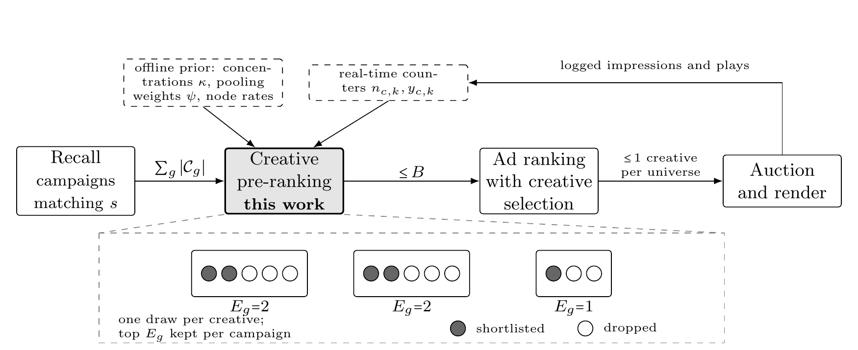
| Step | Where it runs | Output |
|---|---|---|
| Hierarchical prior | Offline batch, refreshed regularly | Shrinkage strength κ per level, attribute pooling weights ψ, each node's play rate |
| Real-time counts | Online, updated per impression | Each creative's impressions and plays split by one attribute at a time |
| Scoring | Online, per request | One Beta posterior per creative, with one draw as its score |
| Truncation | Online, per request | Top E creatives per campaign, at most B in total |
The key division of labor: the slowly drifting prior is computed offline, the fast evidence is read online, and only addition and sampling are left for serving. The parts are explained below.
How much should a new creative borrow from its parents?
The paper puts creatives in a tree: global average, audience segment, advertised game, campaign, creative. Creative B's true play rate is the global average plus one shift per level.
A node with little data cannot trust its own raw rate, so it is shrunk toward its parent's estimate:
Here y is the node's own plays, n its impressions, μ the parent's estimate, and κ the shrinkage strength. Intuitively, κ is the number of impressions at which the node's own data and its parent's view get equal weight.
With the example above (illustrative), suppose the campaign-level estimate μ is 2% and the creative-level κ is 200:
| Creative | Calculation | Shrunk estimate |
|---|---|---|
| B (50 impressions, 2 plays) | (200×0.02 + 2) ÷ (200 + 50) | 2.4% |
| C (no impressions) | (200×0.02 + 0) ÷ 200 | 2.0% |
B's 4% is pulled back to 2.4%, because 50 impressions are not yet convincing; C simply inherits the campaign's level. This is classic empirical Bayes shrinkage. The paper proves this weight minimizes mean squared error, and it equals the posterior mean of a Beta prior, so a Beta distribution can be sampled directly later on.
Why does κ need no tuning? The key is estimating how much children of the same parent truly differ. The raw spread of their rates will not do, because it mixes in sampling noise from small impression counts. The paper uses the DerSimonian–Laird moment estimator common in meta-analysis: compute the impression-weighted scatter, then subtract the part that Binomial sampling noise alone would explain; what remains is the true difference. A parent with a single child, or with one impression per child, cannot separate true difference from noise; its weight in the estimator's denominator is exactly zero, so it takes no part in that level's estimate. Once the variance σ² of the children's true play rates is estimated, the level's shrinkage strength is κ = μ(1−μ)/σ² − 1, with μ the parent's play rate. The less the children differ, the smaller σ², the larger κ, and the more a new child should trust its parent. Each level needs one κ, all read off historical logs in closed form, with no knob to tune.
Too many audience combinations: how are counters stored?
The previous step needs a creative's impressions and plays in "this segment". A segment combines K attributes, each with up to m values, so there are m to the power K combinations. Storing a counter per combination per node is infeasible, and each cell would hold too little data to use.
The paper stores only single-attribute counters instead: how many impressions creative B got under "region = North America", how many under "device = phone", only m×K per node. Each attribute bucket first gets a lift: the log-odds difference between the bucket's play rate (first shrunk toward the creative's overall rate to damp small-bucket noise) and the creative's overall rate. When a request arrives, start from the log-odds of the creative's overall rate, add the lift of the bucket matching each of the segment's attributes, and convert back to a probability; that is the estimate for this segment.
Adding them directly has a problem: attributes are often correlated. Region and language overlap heavily, so the "North America" bucket looks good partly because most of its users speak English; add the two lifts and the same signal is counted twice. The paper gives each attribute a pooling weight ψ: 1 when attributes are fully independent, 1/J each when J attributes fully duplicate one another. Reality falls in between, so ψ is fit once offline by a ridge-penalized logistic regression on the full combination data. Combination counts cannot be stored online but are visible in offline logs, a practical split. Against the plain additive model with all weights at 1, the fitted weights cut reconstruction error by about a third.
One more detail: the posterior needs an effective impression count. The attribute buckets contain the same impressions, so they cannot be summed. The paper takes the minimum over the buckets, because the segment's true impressions cannot exceed any one of them. With the segment's estimated play rate p and effective impressions n, these are converted into n×p plays and n×(1−p) non-plays and combined with the prior, giving Beta(κμ + n·p, κ(1−μ) + n·(1−p)). Its mean is exactly the shrinkage formula above, with μ the parent's estimate.
Why sample instead of ranking by the mean?
With a Beta posterior for each creative, scoring uses Thompson sampling: every request draws one independent sample per creative and ranks by it. Creative C has no data, so its posterior is wide and occasionally yields a high draw, giving it a chance to reach the ranker; creative A has a lot of data, so its posterior is narrow and its draws stay near 2%. The more uncertain a creative is, the more often it gets explored, and the posterior sets that rate automatically, with no separate exploration rate.
Truncation is simple too. Each campaign's quota is its number of creatives times a fraction ρ, rounded down, with a minimum of 1. When the total exceeds the cap B, slots are handed out by round robin, one per campaign per pass. Round robin costs only O(B), and an advertiser cannot gain share by uploading more creatives.
Results
The experiment replays a few hundred Roblox ad requests covering more than 100,000 campaign recalls. For each request, the posterior is rebuilt from the counter state production actually held, and every rule reselects from the same candidates. The evaluation works like this: for each campaign, the most accurate deployed ranker scores the creatives it was sent, and the highest predicted play-through rate among them is that campaign's score, because the ranker keeps only one creative per game in the end. Scores are averaged over all campaigns with at least two creatives and compared with Uniform's average to give the lifts in the table.
The compared rules: Uniform sends one random creative per campaign; TS-One sends the creative with the highest draw per campaign; RR-Random uses the same quota and round robin but picks creatives at random; TS-RR is the full method; Oracle sends every creative to the ranker as an upper bound.
| Method | Mean creatives sent to the ranker | Lift over Uniform | Share of the upper-bound gain |
|---|---|---|---|
| Uniform | just under 500 | — | 0.0% |
| RR-Random | 600 | +2.80% | 15.3% |
| TS-One | just under 500 | +6.09% | 33.2% |
| TS-RR | 600 | +8.14% | 44.3% |
| Rank by mean | 600 | +9.51% | 51.8% |
| Oracle | more than 1,000 | +18.36% | 100% |
The table separates two effects. RR-Random and TS-RR have identical slots and differ only in the score that picks creatives, and their confidence intervals do not overlap, so the gain comes from the posterior itself and extra slots cannot buy it. TS-One sends not a single extra creative and still more than doubles RR-Random's lift.
On cost, scoring every recalled creative takes 79 microseconds, and the whole pre-ranker including truncation takes 2.2 ms. TS-RR's full pipeline takes 41.6 ms against RR-Random's 41.5 ms, a 0.2% difference; Oracle needs 83.1 ms. So the pre-ranker's compute is negligible next to what the ranker spends per extra candidate.
Repeating the evaluation with another deployed ranker, TS-RR recovers 44.0% of the upper-bound gain, almost the same as the main 44.3%. When the quota is tight (ρ=0.2), random picking gains almost nothing (+0.02%) while TS-RR still gains +3.34%, which means the tighter the budget, the more choosing the right creative matters.
Limitations as I see them
First, the value of exploration is invisible in this evaluation. Ranking by the mean earns 1.37 points more than sampling, because the replay is frozen: showing a creative does not change its counters. The authors say 8.14% is a lower bound online, which is reasonable, but how much exploration adds online is something you would have to measure in your own A/B test.
Second, the creative pools are shallow. A campaign has 2.6 creatives on average and over half have only 2, so pre-ranking is mostly a choice between two. When AI generates dozens of creatives per campaign, the posterior and the truncation rule may behave differently.
Third, the metric is the ranker's predicted play-through rate, not real behavior. If the ranker itself is biased on new creatives, the evaluation inherits that bias.
How a recommendation or ads team could try it
- Compute κ per level offline first: take a week of logs, layer by advertiser, campaign and creative, and run the moment estimator for each level's shrinkage strength. The creative-level κ tells you roughly how many impressions a new creative needs before it stands on its own data.
- Add a pre-ranking layer that uses only the shrunk mean ahead of the current creative selection, and compare the ranker's predicted scores against random picking, to check whether the hierarchical prior helps by itself.
- Then switch to Thompson sampling and run a small-traffic A/B, watching the impression share of new creatives and their real click rate once they have enough data; that is the true value of exploration.
- When there are many audience attributes, add single-attribute counters and pooling weights, checking first how correlated the attributes are; only strongly correlated attributes are worth fitting ψ for.
Verdict
The main takeaway: the layer that decides what reaches the ranker also decides what the system can ever learn, and using a point estimate there means giving up on new creatives.
| Dimension | Assessment |
|---|---|
| Problem importance | High. AI generation makes creative counts explode, and creative cold start hits every ads system |
| Method novelty | Medium. Shrinkage, moment estimation and Thompson sampling are classic; the novelty is combining them into a form that runs online in milliseconds |
| Evidence | Medium. The replay is clean and the compared rules isolate each part well, but the main evidence is still an offline replay |
| Engineering cost | Low. Offline is group-by sums; online is a weighted sum and a Beta draw |
| Worth trying | Yes. Any setting where a campaign has several creatives and only one or two can reach the ranker can adopt it directly |
How did this read for you?
Hoot made a note. Thanks for the feedback.

One tap, no sign-in; tap again to undo. Only anonymous counts are kept, never who you are.
Discussion
Add experiment details, reproduction notes or a different take. Requires a GitHub sign-in.
Loading the discussion…