Contents · 9 sections
1What makes the task hard2The overall pipeline3How the slots learn: a coarse outline, slots fill in the details4Making the slots useful for retrieval: two contrastive losses and attention distillation5At retrieval: recall with [EOS], rerank with the slots6Results: ahead on both benchmarks7Limitations as I see them8How a search team could try it9VerdictSHARE

In composed image retrieval, having a multimodal LLM first represent the edited image in a few parts and then gather them into the retrieval vector works better. The task gives a reference image plus a request, such as turning a shirt into a red long-sleeved one, and asks for the image after the change. The usual approach squeezes the reference image and the request into one embedding with a contrastive loss alone. FactEmbed adds a few modification slots near the end of the input, each an extra vector that, after reading the reference image and the request, holds one part of the edited image's details; the last token then gathers them. During training a small decoder gets only these slots and the target image's features pooled into a coarse 2×2 grid, and must fill in the details of every patch. It leads on the main metrics of two standard benchmarks.
Teams building multimodal retrieval, especially "edit this image" search, should read this. The idea is simple: during training an auxiliary task of rebuilding the target image pushes a few slots to each hold a different part of the target, and the later layers of the LLM then gather these slots into the retrieval vector. The extra reconstruction task costs almost nothing at retrieval time, because the decoder is used only in training and each image stores just one more vector. On Refined-CIRR, a version with ambiguous samples removed, R@1 rises from 67.41 for the strongest baseline ReCALL to 68.99.
What makes the task hard
Composed image retrieval takes a reference image and one sentence, and the sentence only says what should change. The model has to work out what to change and what to keep. Here is an illustrative example.
| Content (illustrative) | |
|---|---|
| Reference image | A white short-sleeved shirt with a small logo on the chest, gray wall behind |
| Request | Make it red with long sleeves and drop the logo |
| Image to find | A red long-sleeved shirt, no logo, same cut and collar as before |
| Wrong image that easily ranks high | A red long-sleeved shirt with a completely different collar |
The common approach feeds the whole query to a multimodal LLM, takes the output of the last token ([EOS]) as the embedding, and trains it contrastively against the target image's embedding. The training signal only says "pull this pair together, push that pair apart". Splitting the request into "color changes, sleeves change, collar stays" is left for the model to discover inside a single vector. The authors argue the LLM can already read such requests, and this training setup simply never makes it use that ability.
The overall pipeline
FactEmbed inserts K learnable vectors into the input sequence right before [EOS]. The paper calls them factorized latents; here they are modification slots, with K=8 by default. The query (reference image plus request) and the target image go through the same LLM in two separate passes with shared weights, and each side gets its own 8 slots. The LLM reads front to back and the slots come after the image and text, so each slot can read everything before it; [EOS] comes after the slots, so it can read them.
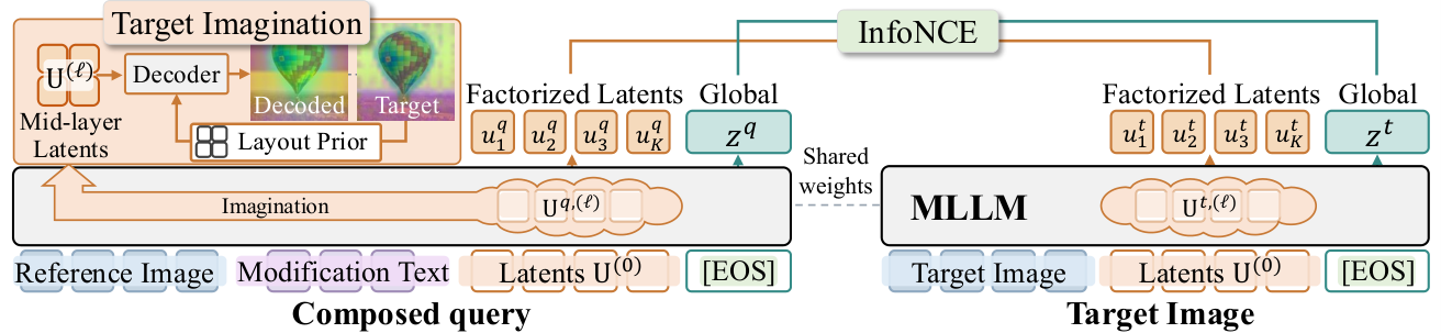
Training and retrieval use different parts, so here they are side by side:
| Phase | What is used | Output |
|---|---|---|
| Training step 1 | Train only the slots and the decoder, with the reconstruction loss only; the decoder gets the target's coarse 2×2 layout | Slots learn to each cover one part of the target |
| Training step 2 | Add DoRA fine-tuning of the LLM and train reconstruction, the two contrastive losses and distillation together | Slots and [EOS] become useful for retrieval |
| Training step 3 | An LLM writes new requests for hard negatives, which become new training samples for one more round | Less noise from sparse labels |
| Retrieval | Run the LLM once, no decoder | One [EOS] vector plus one average of the slots |
Step 3 borrows ReCALL's data augmentation idea, with adjusted details. First it finds candidates the model ranks above the annotated target; the paper calls them hard negatives, and some of them actually satisfy the original request too. An LLM then looks at the correct target image and writes a new request leading from the reference image to such a hard negative, giving a new sample whose answer is the hard negative.
The parts are explained one at a time below.
How the slots learn: a coarse outline, slots fill in the details
Why a decoder at all? If you add a few slots and train them only contrastively, they drift together and collapse into one representation. The appendix measures this: when the slots are trained contrastively alone, the 8 slots of one image have an average pairwise cosine similarity of 0.764; adding reconstruction and distillation brings it down to 0.586, the lowest of the settings tested. Lower means the slots divide the work more clearly.
The decoder is small: one self-attention layer plus a 3-layer MLP, attached to layer 14 of the 28-layer LLM. What it rebuilds is the target image's DINOv2 features, one feature vector per image patch. Each slot is first copied across the whole grid, given position embeddings, and passed through the decoder. For each slot the decoder outputs two things: a grid-sized weight map saying which positions this slot wants to cover, and its guess of the feature at each position.
At any one position, the weights of the 8 slots go through a softmax and add up to 1. Say at the collar position the 8 slots get 0.7, 0.2 and 0.1 shared among the other six (illustrative); the rebuilt feature there mostly follows slot 1. Every position is a weighted sum like this, giving a full rebuilt feature map, which is compared with the target image's real DINOv2 features by mean squared error.
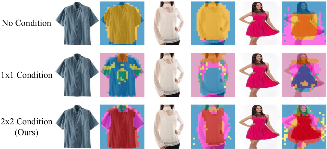
Why give a coarse outline? If the slots alone had to rebuild the whole image, they would spend their effort on large background areas and overall composition, which have little to do with the request. So during training the authors average the target's real features down to a 2×2 grid of four cells, scale it back up, and add it to each slot's input inside the decoder. The query-side decoder also gets this layout of the target image, not of the reference image. This four-cell map only gives the rough layout, so to lower the error further the slots have to supply the details beyond it. The paper's visualizations show that without this map the slots collapse into a few coarse regions; with the 2×2 map, different slots cover local parts such as arms, legs and necklines. Hoot says

No layout map
- decoder gets
- only the slots
- slots must rebuild
- background, layout and neckline, all of it
- result
- slots collapse into a few coarse regions
With the 2×2 layout map
- decoder gets
- the slots plus the target's four-cell coarse features
- slots must rebuild
- details beyond the layout, such as the neckline
- result
- slots each cover arms, legs, necklines
Illustrative: the request turns a round neck into a V-neck. On the left there is no layout map, so the slots must first rebuild the background and overall composition. On the right the target's 2×2 layout is given, the big outline is already there, and the error can only drop if the slots supply details like the neckline. The layout map exists only during training, not at retrieval time. Source: illustrative example for the paper's layout-map design and the Figure 4 visualization (this section)
This is done on both the query side and the target side, and both rebuild the same target image. Inside the LLM, the query-side slots only see the reference image and the request, never the target, so they must "imagine" the target's details on their own; the paper calls this target imagination. The target side does the same, so the slots on both sides split the work the same way and can later be paired across the two sets. One point matters here: the four-cell layout map and the decoder exist only during training. At retrieval time there is no target image and the decoder does not run.
Making the slots useful for retrieval: two contrastive losses and attention distillation
Good reconstruction does not guarantee good retrieval. The slots on the two sides could each be split well yet sit in coordinates that do not line up. The authors add two training terms.
The first is a slot-to-slot contrastive loss, using the slots output by the LLM's last layer. Between the 8 query slots and the 8 target slots, pairwise cosine similarities are computed first, then Sinkhorn optimal transport makes a soft pairing between the two sets: each slot mostly pairs with its closest counterpart and the overall similarity is as high as possible, which gives one total score. Within a batch, this score should be high for the correct query–target pair and low for the others. The [EOS] vector also gets its usual contrastive loss, because it is the vector actually used for large-scale recall.
The second is attention distillation. The decoder sits at layer 14, and deeper layers become more abstract and tend to lose the local split. On the target side, the authors take each slot's attention over the target image's patches at the third layer from the top, and require it to match the weight map the decoder gives that slot, pulled together with a KL divergence. This is done only on the target side, because query-side attention falls on the reference image, whose grid does not line up with the target. The slots and LLM weights are shared by both sides, so the query side benefits indirectly.
The total loss adds three parts: the two contrastive losses (slot-to-slot and [EOS]), the reconstruction loss (weight 1.0) and the distillation loss (weight 0.5).
At retrieval: recall with [EOS], rerank with the slots
At retrieval time one pass through the LLM yields both the [EOS] vector and the 8 slots from its last layer. Storing 8 vectors in the index is too costly, so the authors average the 8 last-layer slots into one vector. Each gallery image stores only two vectors. This average is not optimized directly in training, and used alone for retrieval it gets only 54.87 R@1 on the test set of CIRR (an open-domain composed retrieval benchmark), below [EOS] at 56.12, so it is used only for reranking, not for recall.
First, the [EOS] vector alone finds the top 100 in the whole gallery. Then these 100 are rescored:
Here is the [EOS] vector, is the average of the 8 slots, is the query and is a candidate image. The intuition: [EOS] finds images that match overall, and the slot average restores details that got squeezed out. For example, if candidate A scores 0.80 and 0.60 on the two similarities and candidate B scores 0.82 and 0.50 (illustrative), A's total of 1.40 beats B's 1.32, and A moves ahead of B after reranking.
The extra cost of reranking is tiny. On the CIRR validation set at batch size 1, encoding one query with the LLM takes 353ms, while reranking adds only 0.17ms, under 0.05% of total latency.
Results: ahead on both benchmarks
The main comparison is on Refined-CIRR and Refined-FashionIQ, revised versions with ambiguous samples removed. CIRR has open-domain photos; FashionIQ has clothing.
| Method | Refined-CIRR R@1 | Refined-FashionIQ avg R@10 | CIRR test R@1 |
|---|---|---|---|
| Qwen2.5-VL (same backbone, contrastive only) | 64.64 | 66.82 | 51.98 |
| Qwen3-VL-Embedding 8B | 67.03 | 68.61 | 51.95 |
| CSMCIR (also uses text captions of gallery images) | 67.16 | 69.55 | 53.88 |
| ReCALL | 67.41 | 69.48 | 53.76 |
| FactEmbed | 68.99 | 71.13 | 56.60 |
FactEmbed and ReCALL use the same Qwen2.5-VL-7B backbone. FactEmbed leads on these three main metrics, so the gain does not come from a bigger model. On a few secondary metrics it is slightly behind CSMCIR (a method that also uses text captions of gallery images) or ReCALL, for example Refined-CIRR R@10 is 95.42 against CSMCIR's 95.44.
The ablation takes the parts apart (CIRR test R@1):
| Setup | R@1 |
|---|---|
| Backbone with contrastive training only | 51.98 |
| Add slots and the reconstruction task | 51.45 |
| Add slot-to-slot contrastive loss and attention distillation | 53.28 |
| Add reranking | 54.75 |
| Add the extra data of step 3 | 56.60 |
| Backbone plus step-3 extra data only | 53.69 |
With the reconstruction task alone, R@1 dips slightly, but the FashionIQ validation average R@10 rises from 52.98 to 53.98. The authors explain that reconstruction teaches the slots to split the target image but does not teach ranking, so the contrastive loss and distillation are what turn the split into retrieval ability. For reranking, the paper's combined score Avg. is used, the mean of R@5 and a small-set R@1, where the small set is the 6 candidate images curated for each query. With trained slots, reranking raises the CIRR test Avg. by 1.17; the same reranking applied to slots without the auxiliary training changes it by only -0.37. The reranking gain depends on the trained division of labor, not on simply adding a vector. The extra data alone also helps the backbone, but the full model's R@1 is still 2.91 points higher, so the paper's method and the extra data stack.
Matching all 8 slots with optimal transport gives CIRR R@1 of 56.84, only 0.24 above the reranking version's 56.60, but it needs 8 vectors per image. The reranking version gets most of the gain with two vectors.
Limitations as I see them
First, it is tested only on CIRR and FashionIQ, and the authors themselves say its use as a general multimodal retriever still needs checking. Product search with same-item-different-color cases and fine material details is quite far from these two datasets.
Second, the number of slots is fixed at 8. A request may change one thing or three or four, and the authors acknowledge that the slot count does not adapt to the query.
Third, training adds a whole extra phase over plain contrastive learning. Step 1, which trains only the slots and decoder, takes about 13 hours on 4 RTX PRO 5000 GPUs, and training also needs a DINOv2 encoder to supply the reconstruction target. Retrieval is cheap, but the added training complexity is real.
How a search team could try it
- Add a few learnable vectors to an existing multimodal embedding model and train only the slot-to-slot and [EOS] contrastive losses, then check whether recall moves. This is the cheapest step and shows whether the backbone has headroom.
- Then attach a small decoder, use off-the-shelf visual features such as DINOv2 as the reconstruction target, and add the 2×2 layout map. Check whether the similarity among one image's slots drops clearly, to judge whether the slots really split the work.
- In production, store just one extra average vector and rerank the top 100 of your existing recall. Compare R@1 and latency before and after to confirm the gain holds on your own gallery.
Verdict
The takeaway from FactEmbed: a retrieval vector does not have to be squeezed out by a single contrastive loss. An auxiliary task of rebuilding the target image can make a few slots each cover one part of the target, and the later layers of the LLM then gather them into the retrieval vector.
| Dimension | Assessment |
|---|---|
| Problem importance | Medium-high. Edit-by-image search is in demand on e-commerce and content platforms |
| Novelty | Medium-high. Rebuilding the target constrains each slot's role without extra labels |
| Evidence | Fairly strong. Same-backbone comparison, step-by-step ablation and a reranking control |
| Engineering cost | Medium. One extra training phase and a decoder; one extra stored vector per image at retrieval |
| Worth trying | Yes. Teams with a multimodal embedding model can start with slots and reranking |
How did this read for you?
Hoot made a note. Thanks for the feedback.

One tap, no sign-in; tap again to undo. Only anonymous counts are kept, never who you are.
Discussion
Add experiment details, reproduction notes or a different take. Requires a GitHub sign-in.
Loading the discussion…