SHARE

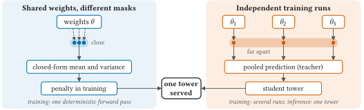
CTR models such as FinalNet and QNN (a quadratic neural network) add a loss on top of the label loss that pulls the network toward its own averaged prediction. For example, the same network runs twice under two dropout masks, and both runs are trained toward their average. The trick works, but nobody has said clearly what it constrains. This paper, by authors at the National University of Singapore and USTC, gives the answer: as the number of masks goes to infinity, such an objective equals exactly "the label loss of the averaged score" plus a penalty on "the disagreement among the masked predictions". When the network structure meets three conditions, this penalty can be approximated in one deterministic forward pass, with no sampling. On that basis the authors design a single-tower model, FLMNet, and then distill towers trained from several random seeds into one student. On five public benchmarks the two FLMNet versions take the top two places in both AUC and Logloss. The absolute gains are small: on Criteo, AUC rises from the strongest baseline's 0.8156 to 0.8169. But the paper breaks down clearly where the gains come from.
1. The question: what does self-distillation actually constrain
FinalNet averages the logits of two interaction blocks and trains each block toward the average. QNN runs one network twice under independent dropout masks, freezes the average of the two predicted probabilities as a target, and pulls both runs toward it. In both, the "teacher" is an average over members of the model being trained, and no second model is needed at serving time; the authors call this family self-ensemble distillation.
Ablations in both original papers show that removing the term lowers AUC, but not by much. QNN drops only 0.06 percentage points on Criteo, and 0.17 and 0.19 on the smaller Frappe and KKBox; FinalNet drops 0.03 to 0.12. The two papers also explain it differently, one as knowledge shared between blocks and the other as mutual correction between runs that smooths the decision boundary, but neither has an experiment that isolates the mechanism.
There is another easy confusion. Members of a classical ensemble are independently trained networks from different initializations or data orders; members of a self-ensemble are just variants of one set of weights under different masks. The former sit in different "valleys" of prediction space, the latter all near one solution. The paper's approach is to treat these two disagreements separately: disagreement inside one tower is called mask noise, and disagreement between seeds is called seed noise.
2. The objective under infinite masking: label loss plus a disagreement penalty
Let a sample's logit under mask be , and the mean logit over all masks be . Cross-entropy can be written , where is softplus; the second term is linear in the logit and produces no extra term when averaged. So after taking the expectation over masks, the loss equals the cross-entropy of the mean logit, plus the term
This is the Jensen gap of softplus: the more the predictions agree, the smaller . The paper proves that when the teacher is pooled in logit space, as the number of masks goes to infinity the self-ensemble objective converges to , up to a term with zero gradient. Ordinary dropout training is exactly ; QNN pooled in logit space has limit . In other words, what self-ensemble distillation adds beyond dropout is just raising the disagreement penalty's coefficient from 1 to 2. Note that the original QNN averages probabilities rather than logits, and this exact result holds only for logit pooling.
is still an expectation over all masks and cannot be computed directly. The authors first bound it: is at most one eighth of the logit variance , and the lower bound degenerates to 0 when the sigmoid saturates. The usual approach is a second-order Taylor truncation that keeps only the term, but on samples with large it underestimates several times over. The paper instead replaces the true mask distribution by a Gaussian of the same variance and evaluates the expectation with three-point Gauss–Hermite quadrature: the function is evaluated only at and and weighted 2/3, 1/6, 1/6, which approximates the expectation under the normal distribution. Compared row by row against a Monte Carlo value from 2,048 sampled masks on trained towers, the ratio of the Gaussian proxy to the true value always stays between 0.72 and 1.12, while the second-order truncation falls below a quarter of the true value on a few samples.
A practical conclusion follows. Keeping only the largest term of the expansion (the term above), is proportional to , and is proportional to ( is the masking rate), so and act only through the "dose" and cannot be identified separately. An ablation that removes the distillation term without adjusting the masking rate changes only the dose, not the form of the objective.
3. A tower structure that makes the variance computable
The Gaussian proxy needs the mean logit and the variance . The authors give three conditions under which both have closed forms: multiplicative gates read only unmasked inputs, the output layer is affine, and each layer only rescales its representation coordinatewise. Then the mean logit equals exactly the logit of the forward pass without dropout, and the variance also has an exact formula. The logit is a bias plus a weighted sum over hidden coordinates, and coordinate 's value is the starting coordinate times the product of the factors each layer applies to it, so its weight is . Each layer's factor is : is this hidden coordinate's own mask factor, is the gate value without masking, and is the perturbation from masking the gate units, computed by multiplying each gate unit's output by its mask factor minus 1 and spreading the result over coordinates through the mixer. So one needs the expectation of the product of any two coordinates and . Since masks in different layers are independent, that expectation is a product over layers: each layer has a hidden-by-hidden table whose entry is , and these entries are multiplied across layers. Here is the variance of a single mask factor and is the gate value; measures how many gate units the two coordinates share, where is the output of gate unit and is the linear layer mixing gate units into coordinates. The extra factor on the same coordinate comes from that coordinate's own mask; different coordinates are linked only through shared gate units. Weighting by and summing gives the second moment of the logit without the bias ; subtracting gives .
QNN-α violates the first condition: its gate reads the masked output of the previous layer, so the random quantities of different layers become dependent. On Criteo, forcing the closed form onto trained QNN-α towers puts the mean more than three standard errors from the sampled mean on 76% to 81% of samples, and after training with the penalty the variance estimate is only 3.6% of the true value. This means training pushes down the estimate rather than the real disagreement. Simply letting the gate read the input embedding makes the formula exact, but lowers validation AUC by 10.5×10⁻⁴ without the penalty.
FLMNet's solution: each field's embedding feeds its own group of ReLU gate units, so no unit sees more than one field; a learnable linear mixing matrix then maps all units' outputs back to the tower's width, giving a gate value for each hidden coordinate, which is how one field's gate reaches every hidden coordinate. The representation is multiplied coordinatewise by . Before entering the tower, the embedding is also recalibrated: in each embedding dimension, the fields' values in that dimension are summed with weights from a learnable field-by-field table, giving the field's adjustment for that dimension, and that coordinate is multiplied by "1 + gain × adjustment". The table compares three towers on the Criteo validation set (mean of three seeds, all with 4 layers and 5 gate units per hidden coordinate, which the paper calls 5 branches):
| Tower | Gate reads | Params | AUC (no penalty) | Closed-form penalty / Monte Carlo value (κ=2) |
|---|---|---|---|---|
| QNN-α | previous layer output | 3.05M | 0.81478 | 0.039 |
| QNN-α reading embedding | input embedding | 3.05M | 0.81373 | 0.998 |
| FLMNet | input embedding, per field | 3.14M | 0.81469 | 1.000 |
FLMNet is only 0.9×10⁻⁴ below the original QNN-α while keeping the formula exact. However, it changes three things at once, and this comparison only shows their combined effect.
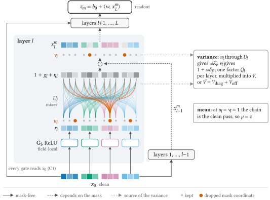
The exact variance needs, per layer, a table the size of the hidden dimension squared, two orders of magnitude more expensive than a forward pass, so it serves only as a ruler. The exact variance has two kinds of terms: those involving a single hidden coordinate, and cross terms linking two different coordinates. Training uses a truncated version: it keeps all of the first kind, and for the second it expands the product over layers as a polynomial in and keeps only the linear term, the part where only one layer's gate masks act at a time, dropping and higher. That costs just two extra matrix multiplications per layer. At the median over 24,576 validation samples, this truncation underestimates the variance by only 0.035%. For comparison, a coarser approximation that also expands the random masks on the gate units only to first order underestimates it by about 8%, which is why the authors use the first one. The appendix also records an engineering lesson. The authors once wrote the variance as the difference of two nearly equal large numbers, got negative variances, and wasted four training runs before finding the cause; they switched to a recursion in which every term is nonnegative.
4. Experiments: how much it gains, and from what
The five benchmarks are Criteo, Avazu, KKBox, Frappe and ML-1M, against seventeen models, all rerun by the authors under one protocol, mostly averaged over three to six seeds. Avazu's original validation and test sets have different positive rates (16.8% vs 15.2%), so the authors pooled them and re-split at random.
| Model | Criteo AUC | Avazu AUC | KKBox AUC | ML-1M AUC |
|---|---|---|---|---|
| DNN | 0.8136 | 0.7578 | 0.8502 | 0.9009 |
| FinalNet | 0.8151 | 0.7607 | 0.8515 | 0.9056 |
| QNN-α two heads | 0.8156 | 0.7568 | 0.8575 | 0.9052 |
| FLMNet-CF | 0.8162 | 0.7617 | 0.8581 | 0.9087 |
| FLMNet-KD | 0.8169 | 0.7620 | 0.8604 | 0.9099 |
CF is the single tower with only the closed-form penalty; KD is a student distilled on top of it from three CF towers. Measured by RelaImpr, the AUC gain over DNN (a plain multilayer-perceptron baseline) divided by DNN's margin above the 0.5 of a random ranker, the five-benchmark average is 1.36% for CF and 1.62% for KD, against 0.66% for the strongest baseline, two-head QNN-α. Before looking at the test set, the authors fixed for each benchmark an opponent (the strongest baseline on validation) and a lead threshold: comparing test AUC seed by seed, the mean difference must exceed twice its standard error (or a preset floor, whichever is larger). Below this is called the seed threshold. CF's lead is 1.9 to 8.7 times the threshold on every benchmark, but with only three to six seeds this is a lead under a pre-agreed rule, not a significance test.
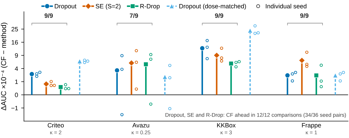
The closed-form penalty is compared with three sampling-based regularizers, all on the same tower: dropout at , the two-pass self-ensemble loss, and R-Drop. Across four benchmarks and three methods, 36 seed pairs in all, the closed-form penalty wins 34. Because dropout's dose is only a half of CF's on Criteo and a third on KKBox, the authors also reset dropout's masking rate to match the dose: 2/11 on Criteo, 1/4 on KKBox and 1/37 on Avazu. On Criteo and KKBox the closed-form penalty still leads on every seed, by 6.5×10⁻⁴ and 23.9×10⁻⁴ on average. On Avazu its lead is only 1.9×10⁻⁴ and changes sign across seeds, suggesting the advantage there may come mainly from dose.
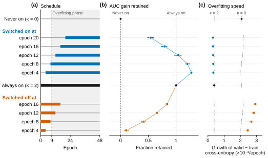
Why does the penalty help? On Criteo with a fixed learning rate, the authors switch the penalty on or off mid-training. While it is on, the gap between validation and training cross-entropy grows by only about 0.3×10⁻³ per epoch, six to seven times slower than with no penalty; once it is off, the gap grows by more than 2.5×10⁻³ per epoch. So the penalty mainly slows overfitting. It also has a cost early in training: switching it on at epoch 4 gives a peak AUC 2.6×10⁻⁴ higher than switching it on from the start, and the run penalized from the start trails the unpenalized run from epoch 2 to 10. This experiment uses one dataset, a fixed learning rate and an onset tested every four epochs, so "epoch 4" should not be taken as a general setting.
On the seed-noise side, by an identity, the amount by which a teacher pooling seeds beats the member average in Logloss equals exactly the Jensen gap between seeds, and it grows as . The student retains about six tenths of it at every . On Criteo, a student distilled from five seeds has AUC 0.80×10⁻³ above a directly trained member, and the teacher itself is 1.44×10⁻³ higher. The student does not start from scratch: it starts from one seed's fully trained model and is then distilled toward the teacher. As a control, continuing from that same starting point with labels only, no distillation, raises validation Logloss by 16×10⁻³, and in parameter space the direction the weights move under label training is nearly perpendicular to the direction they move under distillation, so the two change different parts of the model. The authors read this as the labels having no more generalizable information to give at this point; what remains is fitting to individual samples.
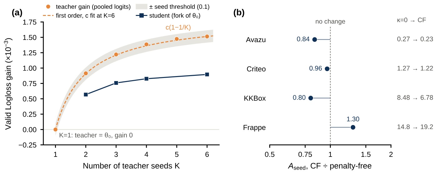
The right panel shows the penalty barely reduces seed disagreement, with ratios between 0.80 and 1.30, and on Frappe it even grows. The two gains therefore largely add up. On Criteo and KKBox, where each single gain exceeds the seed threshold, using both retains 87% and 80% of their sum; on Avazu and Frappe the AUC differences among the four combinations are all within the threshold, so additivity cannot be judged.
On cost, on one V100, CF takes 46.7 ms per step, comparable to QNN-α's 45.4 ms with one head and 47.0 ms with two, because the saved second forward pass offsets the variance computation. But peak memory is about half again as high, 1,667 vs 1,106 MiB. KD needs training runs, and inference latency is about 5.8 ms for all.
5. Limitations
The authors list three boundaries. The three conditions are sufficient, not necessary, for the closed form, so towers outside them need checking; training uses a Gaussian proxy, not the exact Jensen gap; and the gap between seeds has no closed form, so how much distillation recovers can only be measured. Also, the two gains are obtained separately, the penalty within one training run and distillation over .
A few more points are worth noting. On the two advertising benchmarks all models are rerun at embedding dimension 10, and FinalNet and FinalMLP on Criteo come in 3.2×10⁻⁴ and 4.5×10⁻⁴ below their public leaderboard values, which the authors attribute to the leaderboard reporting a single tuned run. FLMNet uses a cosine learning-rate schedule and weight averaging; the baselines do not. KD students share some teachers and cannot be treated as independent repeats. All conclusions come from public offline benchmarks, with no online experiment.
6. Practical implications
If your ranking model already uses a two-pass dropout consistency loss, this paper gives two points you can check directly. First, see whether the teacher is pooled in logit or probability space, and whether gates read masked intermediate states; if the conditions are not met and you force the closed-form variance anyway, the model will "fool" the penalty. Second, when tuning such losses, tune the weight and masking rate together as one dose, and align dose before comparing regularizers, otherwise a difference in strength is easily mistaken for a difference in method.
Multi-seed distillation can be treated as a separate offline investment. It changes neither the structure nor the inference cost, but needs CF teacher runs in total (including the tower the student starts from) plus one student run; for frequently updated models, that training cost and freshness have to be counted together.
How did this read for you?
Hoot made a note. Thanks for the feedback.

One tap, no sign-in; tap again to undo. Only anonymous counts are kept, never who you are.
Discussion
Add experiment details, reproduction notes or a different take. Requires a GitHub sign-in.
Loading the discussion…