Contents · 11 sections
1What problem is it actually solving?2The big picture first: one product, two sets of tools3Single-GPU efficiency: rewriting attention kernels for recommendation data4Why move long sequences to block attention?58-bit precision: the hard parts are quantization overhead and numerical stability6Scaling efficiency: parallelism by network tier, communication off the SMs7Memory and load balancing8Key numbers9The limitations as I see them10How a recommendation team could try this11One-line conclusion and assessmentSHARE

This is worth reading for teams that train large recommendation models, especially if sequences keep getting longer and GPU counts keep growing while training efficiency does not follow. It does not answer "how should the model be designed". It answers a more basic engineering question: recommendation data has wildly varying lengths and half the parameters live in huge sparse tables, so why does an LLM training stack tuned for fixed-length text work poorly, and what has to change. The core idea in one sentence: split end-to-end efficiency into "how full a single GPU runs" times "how much survives when scaling to thousands of GPUs". The first factor is raised with attention kernels written for recommendation and with 8-bit precision. The second is raised with parallelism mapped to network tiers, communication that does not occupy compute units, and data batching balanced by sequence length. Over 12 months total training compute grew 4x while end-to-end MFU doubled to 20% to 25%. This is a Meta engineering blog post, not a paper: there is no ablation table and the gains are measured against different baselines, so read it for the list of methods rather than for an exact accounting of gains.
What problem is it actually solving?
GEM (Generative Ads Recommendation Model) is the foundation model behind Meta's ads recommendations, used for ads ranking on Facebook and Instagram. It has trillions of sparse embedding parameters and billions of dense parameters. Inputs come in two kinds: sequence features such as user activity history, and non-sequence features such as user location and ad creative representations. Each kind goes through its own attention modules, and then they interact.
An illustrative example shows where the trouble starts. A batch holds 4 users whose activity sequences have lengths 100, 300, 500 and 1000 (illustrative). The usual LLM practice pads everything to 1000, so 4000 positions are computed, of which only 1900 are real; more than half the compute goes to padding. The blog's production figure: padding wastes up to 50% of compute.
Without padding, a single GPU saves that compute, but a new problem appears across thousands of GPUs. The total sample length each GPU (a "rank" in the blog) receives changes every step, and the heaviest rank does about 15% more work than average at every step. Distributed training waits for the slowest rank at each step, so that 15% becomes idle time on every GPU.
There are two more recommendation-specific difficulties. First, attention shapes are very asymmetric: self-attention over the activity sequence has long sequences but short windows; user–ad cross-attention has long queries and short keys/values; pooled attention, which compresses a long history into a few vectors, has short queries and long keys/values. Kernels tuned for long LLM sequences cannot keep their pipelines full on these shapes. Second, ads objectives such as CTR and CVR are very sensitive to numerical error, so simply lowering precision easily hurts quality.
The big picture first: one product, two sets of tools
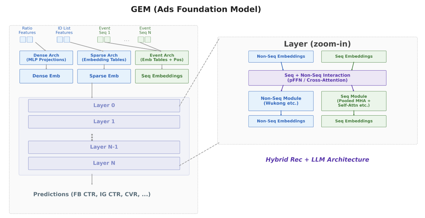
The blog organizes all the work around one formula:
Local MFU is single-GPU efficiency: run each layer of the model alone on one GPU, with no communication or recomputation, and see what fraction of hardware peak is used. Scaling Ratio is scaling efficiency: end-to-end MFU divided by Local MFU, where 1.0 means perfectly linear scaling. An illustrative example: if one GPU reaches 40% and only 55% of that survives at thousands of GPUs, end-to-end MFU is 22%. The benefit of this split is that you can measure separately whether a change improves the single GPU or the scaling.
| Problem | Which factor | Tool |
|---|---|---|
| Padding waste, asymmetric shapes | Single-GPU efficiency | Three kinds of kernels: JFA, GDPA, BlockAttention |
| Low precision saves compute but risks quality | Single-GPU efficiency | MXFP8 attention and MLP, plus numerical-stability measures |
| Heavy communication, low cross-machine bandwidth | Scaling efficiency | 5D parallelism laid out by network tier |
| Communication kernels compete for compute units | Scaling efficiency | Move data with dedicated hardware instead of the GPU's compute units (SMs) |
| Memory pressure forces recomputation | Scaling efficiency | Per-region automatic recomputation budgets + activation quantization |
| Uneven load across GPUs | Scaling efficiency | Base Batch Shuffling |
The sections below take this table apart.
Single-GPU efficiency: rewriting attention kernels for recommendation data
The first kernel is JFA (Jagged Flash Attention, a FlashAttention that works directly on variable-length sequences). It does not pad; it computes directly on tensors of uneven length. JFA went through four generations, from slower than the padded standard implementation to matching hand-written CUDA. One change deserves a closer look: how sequence boundaries are handled.
The usual approach builds a 2D mask and fills out-of-bounds positions with negative infinity; these element-wise operations took about 28% of executed instructions. JFA instead sets out-of-bounds queries and keys to zero, which TMA (the GPU hardware unit dedicated to moving tensor data) does for free, without compute instructions. A zeroed key has a dot product of 0 with any query, so the softmax denominator gains an extra . As I read it, "subtracting the extra exponents" means removing this term from the denominator. Worked by hand: real scores are 2 and 1, plus a zeroed position scoring 0, so the denominator is ; subtracting gives 10.11, exactly what the real positions alone produce. The blog says the two approaches are numerically equivalent, and the 28% of masking instructions disappears. JFA v4 delivers 40% to 140% more floating-point throughput than v2, giving an 18.5% relative gain in single-GPU MFU and a 12% QPS gain.
The second kernel is GDPA (Generalized Dot-Product Attention). GEM's self-attention, pooled attention and cross-attention are all "two matrix multiplications with an element-wise activation in between", except that the activation is GELU or SiLU instead of softmax, so one kernel can cover them all.
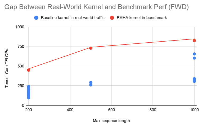
Why write a separate kernel? The figure above shows the issue: the same class of kernel runs well on a standard benchmark and drops a lot on real traffic. The blog measured a 2.6x forward gap, 4x in the worst case. The reason is that keys/values are short, the inner loop runs only 1 to 2 iterations, and a pipeline designed for long sequences never gets going. GDPA does three things.
First, without softmax there is no softmax correction stage, which frees 4 warps (a warp is a group of 32 GPU threads that execute together) and their registers. A FlashAttention-style kernel processes each query block by reading key/value blocks one at a time in an inner loop, overlapping data movement and compute by "prefetching the next block while computing this one". With short keys/values the inner loop runs only 1 to 2 times, so there is no next block to prefetch. As I read it, GDPA overlaps at the outer loop instead: while computing the current query block, it prefetches the data for the next query block, recovering about 10% of performance.
Second, attention is split into many small compute blocks of "a span of queries × a span of keys", called tiles; in the padded region of variable-length sequences, some tiles are entirely empty. GDPA first computes on the CPU which tiles contain valid data and skips empty ones, then interleaves the remaining tiles across SMs (streaming multiprocessors, the GPU's compute units) so that the tiles of long samples do not pile up on a few SMs. The blog calls this zigzag assignment; the effect is that per-SM load skew drops from 6x to near balance.
Third, the tanh inside GELU needs the GPU's scarce special-function units; GDPA replaces it with a 6th-order Taylor expansion that uses only ordinary arithmetic units. A Taylor expansion is accurate only when the input range is bounded, and QK-norm (normalizing queries and keys) guarantees exactly that.
The result is a 2x forward speedup at about 97% Tensor Core utilization, which shows that even short, asymmetric shapes can nearly saturate the hardware; backward is 1.6x faster. With short keys/values it is up to 3.5x faster than FlashAttention 4 on the forward pass, meaning general-purpose kernels really do lose out on these shapes. Applied across the full model, these kernels raise training throughput by more than 30%.
Why move long sequences to block attention?
The cost of full self-attention grows with the square of sequence length. GEM first moved to sliding-window attention, where each position only looks at nearby events and cost becomes "length × window". Long-sequence self-attention latency dropped by up to 68% with neutral NE (normalized cross-entropy, Meta's usual model-quality metric).
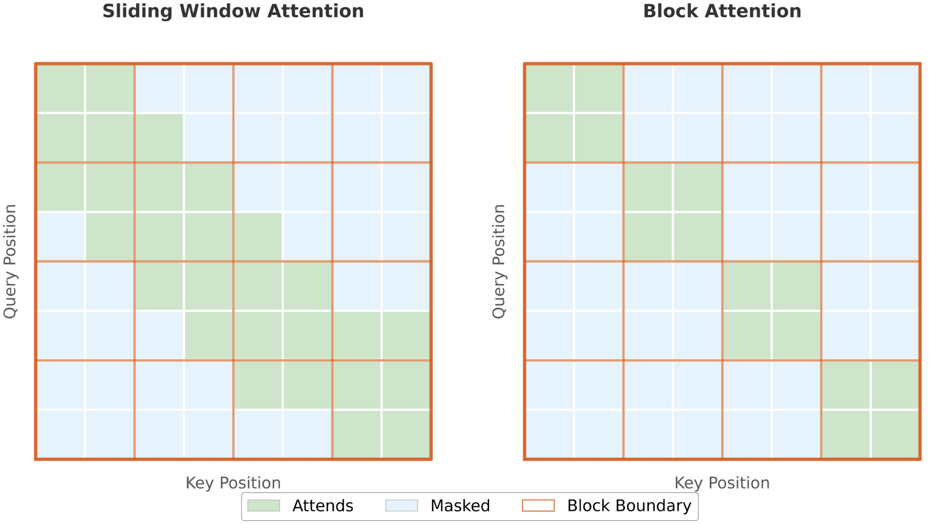
Then GEM went further: fixed 64-token blocks, with each query block attending only to its matching key/value block, so attention becomes many independent 64×64 problems. Worked by hand: at sequence length 1024, full attention computes about 1.05 million query–key pairs; cut into 16 blocks it needs only 16×64×64 ≈ 66 thousand, 1/16 of the original. It saves more than the sliding window because there is no partial-window masking inside a block and no iteration over multiple tiles, so FlashAttention overheads such as online softmax correction and writing logsumexp back to memory can be dropped. With RoPE's backward pass also fused into the attention epilogue, self-attention layer MFU is 30.6% higher than Triton block attention and about 44% higher than the sliding window.
The blog says GEM "could safely" use 64-token blocks; the only step in the post reported with an NE number is the sliding window. Blocking means events on either side of a block boundary cannot see each other, and whether that is harmless for your sequences is something to verify yourself.
8-bit precision: the hard parts are quantization overhead and numerical stability
On the latest-generation GPUs, FP8 peak compute is 2x FP16 and FP4 is 4x. But low precision is not a data-type swap: quantization itself costs compute and memory traffic and can eat the savings, and recommendation objectives are sensitive to numerical error. GEM uses MXFP8 (an 8-bit floating-point format in which each small block shares one scale factor).
Why scale per block? 8 bits cover a narrow range; the largest value in a block decides how the block is scaled, and smaller blocks are less likely to be dragged by a few large values. GEM uses 32×32 square blocks with one scale factor each. Square blocks stay the same block with the same factor after transposition, so each tensor is quantized only once and the backward pass, which needs transposed Q and K, simply reuses it.
Quantization overhead is removed by fusion. Weights are quantized on each rank's local FSDP shard before the all-gather, so 8-bit data is sent, no rank re-quantizes the full weight, and communication volume shrinks. Activation quantization is fused into the preceding normalization and projection kernels, so attention consumes 8-bit input directly with no extra memory round-trip. Numerical stability rests on three things. The first is a random Hadamard transform before quantization. A normalized Hadamard matrix satisfies , so the matrix product can be rewritten as with the same result, while spreads a few large values in a row across all columns. An illustrative hand calculation: the row [8, 0, 0, 0] times the normalized 4×4 Hadamard matrix becomes [4, 4, 4, 4], and the maximum drops from 8 to 4, so per-block scaling is not dragged by one large value; "random" means the signs of the columns are also flipped at random. The second is stochastic rounding, which removes the bias of always rounding in one direction. The third: weight gradients have more severe outliers, so low precision is skipped for them or higher precision is used. The later layers, which are more sensitive to error, stay in BF16. On representative shapes, the MXFP8 forward kernel is more than 1.3x faster and backward more than 1.5x faster. The blog describes the quality effect as "no quality regression".
Scaling efficiency: parallelism by network tier, communication off the SMs
Meta's training cluster has three network tiers: the 8 GPUs in one machine use NVLink, machines within one AI zone use RoCE (RDMA over Ethernet), and links across zones also use RoCE, but the total cross-zone bandwidth is less than the sum of the machines' bandwidth, so machines share it and the usable bandwidth is clearly lower. The design rule: when communication on one tier becomes the bottleneck, add a parallelism dimension that makes messages on that tier smaller or involves fewer GPUs.
Dense parameters use three dimensions. FSDP shards and gathers parameters only within groups of 128 to 256 GPUs, and between groups, as in DDP, only gradients are all-reduced. Because parameters are already split into many pieces, each GPU only synchronizes its own small piece, so the low cross-zone bandwidth is tolerable. Illustratively: 4096 GPUs split into 32 groups of 128 gather parameters within 128 GPUs rather than across all 4096. Large DHEN (Deep Hierarchical Ensemble Network) expert modules have so many parameters that prefetching cannot hide their communication, so expert parallelism is added: each GPU holds only one expert, and FSDP only needs to gather that one expert's parameters, so messages get smaller. In the configuration the blog gives, two GPUs in the same machine each hold one expert, forming 2-way expert parallelism; each expert's parameters are further sharded with FSDP across 16 machines (16-way). Before computing, each GPU gathers its expert's parameters across machines, then exchanges activations with the other GPU in the same machine over NVLink, so each expert processes all samples from both GPUs, and the results are sent back afterwards.
Sparse parameters went through three generations. The first sharded embedding tables across all GPUs; with too many GPUs, each got too few tables to balance, and every all-to-all involved everyone. The second split GPUs into groups of about 256; within a group the full set of embedding tables is sharded so each GPU stores one piece and the group together stores a full set, with data parallelism across groups. All-to-all happens only within a group, which improves load and communication, at the cost of one full copy of trillions of parameters per group. The third splits each GPU's piece of the tables again across several GPUs in the same machine. The blog only says the new all-gather and reduce-scatter both run on intra-node NVLink; as I read it, this adds one more level of sharding inside the machine: before a lookup, the piece is temporarily reassembled within the machine, released before peak memory, and overlapped with dense compute. The blog's verdict on this generation is that sparse scaling becomes nearly overhead-free.
Communication kernels themselves occupy SMs: all-gather and reduce-scatter each take about 24 SMs, costing up to 15% efficiency. Meta's NCCLX (Meta's own extension of NCCL) moves intra-node traffic with the copy engine and inter-node traffic with RDMA, cutting all-gather's SM usage from 24 to 1 and raising end-to-end QPS by about 5%.
Memory and load balancing
Once parameters are sharded, each GPU's memory is dominated by activations. PyTorch's compiler-based automatic recomputation used to apply one memory budget to the whole model; GEM switched to per-region budgets. When the PyTorch compiler hits code it cannot compile it breaks the computation graph (a graph break), and a region is the subgraph compiled between two breaks; each region gets its own budget, and memory goes first to the regions where "each GB of activations saves the most recomputation time". On top of that, activations saved for the backward pass are quantized from BF16 to FP8 or MX4 (the 4-bit format of the same family). With this, each GPU's local batch can exceed 1000 samples with modest recomputation cost.
Load imbalance is handled by BBS (Base Batch Shuffling). Global balancing needs GPUs to exchange samples every step, adding an all-to-all whose communication eats the savings. Balancing within one GPU needs no communication; the blog's comparison table rates its balancing quality at "90% of optimal"; read it as capturing most of the benefit of ideal balancing. BBS is of the second kind. The blog's description: each GPU's data reader generates sub-batches of 128 samples, sorts them by total sequence length within the sub-batch, and when merging them into full batches (1000-plus samples per GPU) pairs the heaviest with the lightest in turn, so one full batch is made of 8 or more sub-batches. As I read it, you can do this: collect the sub-batches needed for several full batches, sort them, take one from each end to form a pair so that every pair has a similar total length, then hand the pairs out to the full batches in turn. Illustratively: 16 sub-batches with total lengths 16, 15, …, 1 form eight pairs 16+1, 15+2, …, 9+8, each summing to 17; each full batch takes 4 pairs, i.e. 8 sub-batches, so both batches total 68 and neither is especially heavy.
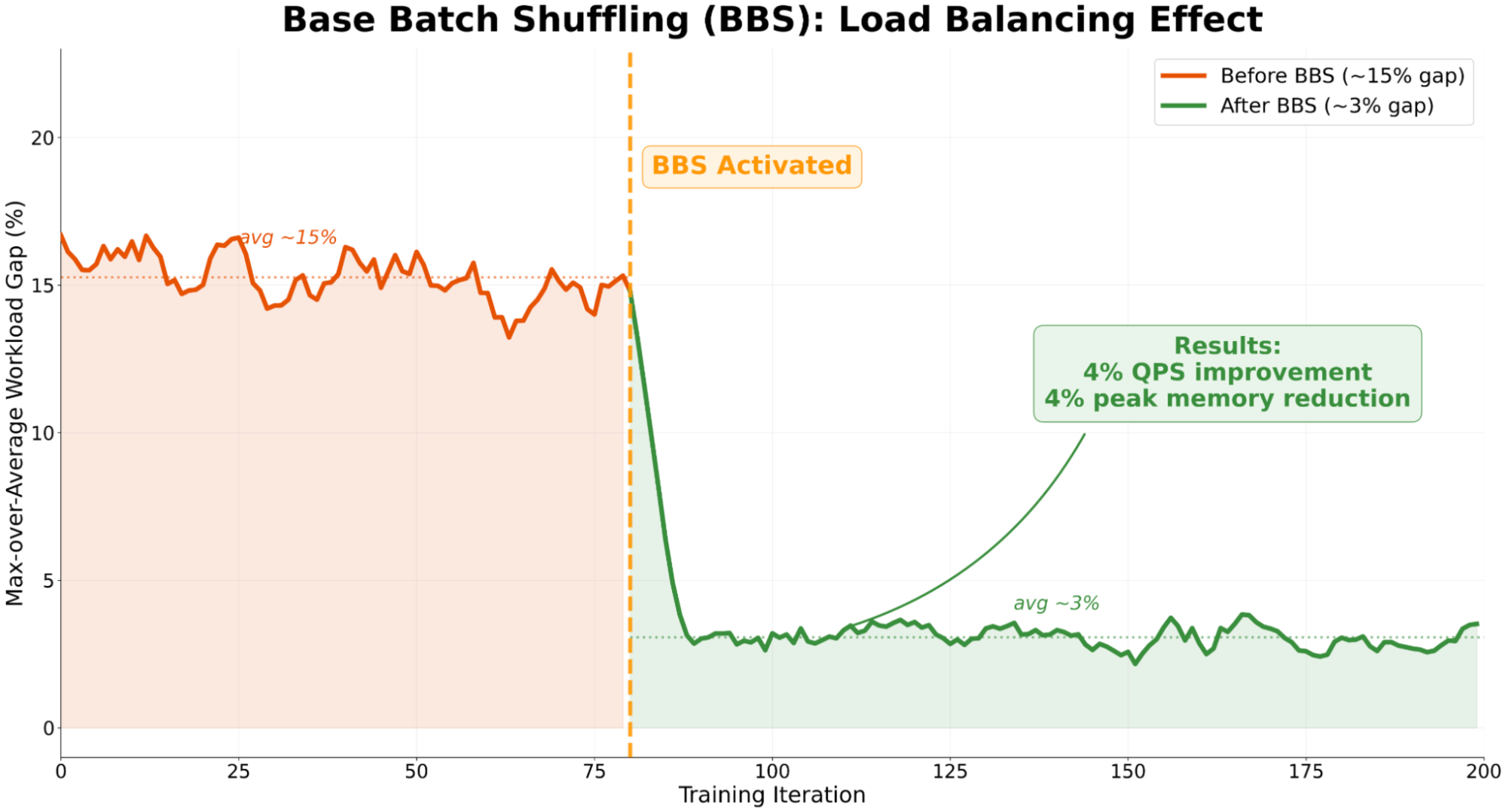
This shows that without any cross-GPU communication, just by changing how batches are formed when reading data, the drag of the slowest GPU falls from about 15% to about 3%. This is the easiest item in the post to copy, and it applies to any unpadded variable-length sequence training.
Key numbers
| Technique | Compared with | Result |
|---|---|---|
| JFA v4 | JFA v2 | TFLOPS +40% to 140%, single-GPU MFU +18.5% relative, QPS +12% |
| GDPA | Original kernel | Forward 2x (1145 TFLOPs), backward 1.6x, full-model throughput +30% or more |
| Sliding-window attention | Full self-attention | Long-sequence latency up to −68%, NE neutral |
| Block attention + fused RoPE | Sliding window | Self-attention layer MFU about +44% |
| MXFP8 attention | BF16 | Forward more than 1.3x, backward more than 1.5x |
| NCCLX SM-free all-gather | Standard NCCL | SM usage from 24 to 1, end-to-end QPS about +5% |
| BBS | No balancing | Load gap from about 15% to about 3%, QPS +4%, peak memory −4% |
| Overall | 12 months earlier | Total training compute ×4, end-to-end MFU doubled to 20% to 25% |
Every row in this table has a different baseline, some a previous kernel, some a standard benchmark, so the percentages cannot be multiplied or added up to reproduce the "doubling".
The limitations as I see them
First, the gains cannot be accounted for. Each gain has its own baseline, so neither each item's share of the overall doubling nor how far Local MFU and Scaling Ratio each moved can be derived from the numbers in the post, which is exactly the question its own decomposition should answer.
Second, the quality evidence is thin. Only sliding-window attention is explicitly reported as NE-neutral; MXFP8 is only described as having "no quality regression", and block attention as "safe to use", both without numbers. Sensitivity of CTR and CVR to precision is the very risk the blog itself stresses.
Third, transferability is limited. Many gains rely on latest-generation GPU features (TMA, MXFP8 instructions) and on Meta's internal NCCLX and three-tier network. Teams with a few hundred GPUs of an older generation can mainly reuse unpadded variable-length kernels, block attention and BBS-style batching.
How a recommendation team could try this
- Measure two numbers first: the fraction of compute lost to padding, and how much more the heaviest GPU does than average each step. If the first is large, variable-length kernels are worth it; if the second is large, start with batch balancing.
- The cheapest step is BBS-style batching: sort by total sequence length when reading data and alternate heavy and light when forming batches. It only changes the data pipeline, not the model; check whether the gap between maximum and average step time narrows.
- Try sliding-window or block attention on long activity sequences while watching offline AUC or NE, especially whether block boundaries cut off useful recent behavior.
- Apply low precision first only to large matrix multiplications, keep later layers and weight gradients in BF16, and widen the scope only after comparing loss curves and offline metrics.
One-line conclusion and assessment
The thing most worth taking away: training efficiency for recommendation models has to be accounted for in two ledgers, single GPU and scaling, and variable-length sequences waste resources in both; on one GPU the fix is not padding, across many GPUs it is balanced batching.
| Dimension | Assessment |
|---|---|
| Problem importance | High. As recommendation models scale toward foundation-model size, training efficiency decides how far they can scale |
| Method novelty | Medium-high. The subtraction masking in the variable-length kernel, GDPA unifying non-softmax attention, square-block quantization and BBS are concrete designs for recommendation data |
| Experimental evidence | Medium-low. All production measurements, no ablations, inconsistent baselines, and most quality effects have no numbers |
| Engineering cost | High. Most kernels depend on the newest hardware and an internal communication library; BBS and block attention are cheap |
| Worth trying? | Yes. Start by measuring load gap and padding ratio, and do BBS first |
| Where it fits | Recommendation models whose user activity sequences vary a lot in length, trained on hundreds to thousands of GPUs |
How did this read for you?
Hoot made a note. Thanks for the feedback.

One tap, no sign-in; tap again to undo. Only anonymous counts are kept, never who you are.
Related papersMore from Paper Daily
 Personalization · 2026-10-29Meta Andromeda: Powering the Next Generation of Ads Retrieval Through Model-System Co-DesignMeta's next-generation ads retrieval engine Andromeda brings near-ranking-quality models to retrieval, scoring every eligible ad. The new version replaces the single user tower with several specialized user towers as experts, and encodes the ad tower with real-time request context. An attention-based gate in the interaction layer activates only the most relevant experts per ad, cutting inference…
 Generative · 2026-07-29Realizing Scaling Laws in Recommender Systems: A Foundation-Expert Paradigm for Hyperscale Model DeploymentDeep dive: Realizing Scaling Laws in Recommender Systems: A Foundation-Expert Paradigm for Hyperscale Model Deployment.
 Personalization · 2026-11-04Auditing Representation-Space Fraud Detection: A Bayesian IRL Framework for Calibrated Uncertainty and Its LimitsShilling detection almost always reports a single AUROC, and that number cannot say when the detector can be trusted. This paper builds an auditing framework to check exactly that. Common fake-account injections are all caught. An attack that copies real users changes everything: each fake account copies every movie a real user rated and adds 1 to 3 target movies, and on MovieLens-1M AUROC falls…
Discussion
Add experiment details, reproduction notes or a different take. Requires a GitHub sign-in.
Loading the discussion…