Contents · 9 sections
1What problem is it actually solving?2Does scaling help? Per-task scaling-law fits3Making a 1B model retrainable: sampled softmax and a projected decoding head4Labels go stale under cached serving: multi-token prediction (MTP)5Cold start: semantic towers plus ID masking6Production-shadow results7Limitations as I see them8How a recommendation team could try it9Conclusion and assessmentSHARE

Teams building industrial generative recommenders and weighing whether to make the model bigger should read this. It is an experience report from Netflix, not a new-architecture paper. They scaled a generative recommender's backbone from 2M to 1B parameters and found that the gains differ by task. They then used a scaling law with a ceiling to judge which kinds of task still merit more parameters, and paired the scale-up with three engineering changes so the large model can be retrained repeatedly, match cached serving, and score new titles. In a one-week production-shadow evaluation over 1M users, the 1B model raises MRR by 22.5% relative on long-horizon taste tasks (Task A) and by 28.1% on cold-start titles, but only by 7.4% on time-driven tasks (Task C). The most useful parts, in my view, are two lessons: scaling laws can serve as a diagnostic for "should we keep adding parameters", and cached serving makes next-token labels stale. But the shadow result compares the scale-up bundled with three other changes, so it cannot be read as "scaling gave 22.5%".
What problem is it actually solving?
Netflix's model compresses each user event's action, viewing context and title metadata into one token and is trained to predict later events. The appeal of this kind of model is that one backbone can serve many downstream tasks at once: retrieval, ranking features, user embeddings, cold-start scoring. But in production, "better pre-training metrics" does not automatically become "better downstream recommendations". The authors name four sticking points. Does the task itself still have headroom? Does training cost hold up when trillions of behavior tokens must be retrained on a fixed cadence? Does the training target match the actual serving moment when results are cached to save money? Can the model score newly launched titles that have no reliable collaborative ID embedding yet?
A running illustrative scenario: a user watched episode 3 of a crime drama last night. The recommender computes and caches their recommendations overnight, and the cache is only used when they open the home page the next evening. Under next-token training, the "right answer" the model learns is episode 4, but by serving time they have quite possibly watched episode 4 on the commute, and what should be recommended is episode 5, or another series in the same genre. Meanwhile, the platform launched a new series that day with almost no viewing history. The paper's changes each address a different problem in this scenario.
Does scaling help? Per-task scaling-law fits
The authors first group Netflix recommendation scenarios coarsely into three task categories, to avoid exposing internal surface names:
| Task | Predictability | Meaning |
|---|---|---|
| Task A | Lower | Long-horizon taste; sparse positives; target may extend beyond the current session |
| Task B | Moderate | Short-horizon engagement; recent actions and session intent are more informative |
| Task C | Higher | Driven by launch timing, catalog availability, broad popularity |
The setup is a time split: user history ends before a cutoff, and labels come from real behavior after it. Models of different sizes share the same training data, evaluation examples, item vocabulary, embedding dimension and decoding setup; only backbone size changes, and parameter counts exclude embedding and decoding layers. The metric is MRR, because it is continuous and bounded by 1, which suits fitting a curve that approaches a ceiling.
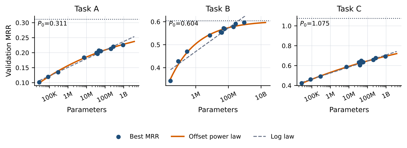
The fit is , where is the fitted saturation level. The three tasks come out very differently. Task A has of 0.311, while MRR at 1B scale is only around 0.22, still far from the ceiling. Task B has of 0.604, already close to the best value observed in this scale range. Task C has of 1.075, above MRR's theoretical maximum of 1, and the authors acknowledge the excess as estimation error. Compared with the log-linear fit used by HSTU, the offset form has lower fit error on all three tasks:
| Task | Offset power-law RMSE (×10⁻³) | Log-linear RMSE (×10⁻³) |
|---|---|---|
| Task A | 2.80 | 5.43 |
| Task B | 8.16 | 21.34 |
| Task C | 9.33 | 10.97 |
This shows that “does adding parameters help” has to be asked per task. For a task like Task B that is already near its ceiling, further backbone scaling will pay off little, and the objective or serving path is the better thing to change; for a task like Task A that is far from its ceiling and matters to the product, scaling still has room. The authors also stress that is a diagnostic under the current data, objective and evaluation distribution, not a measure of the task's value.
Making a 1B model retrainable: sampled softmax and a projected decoding head
One difference between recommenders and language models is that recommenders must be retrained often, because tastes, seasons and the catalog change every day. The authors' pre-training data has 2 trillion behavior tokens per cycle. At this scale, an output layer that scores every candidate item directly takes a large share of training cost: the more candidate items, the bigger the output-layer matrix multiply, while backbone compute stays the same.
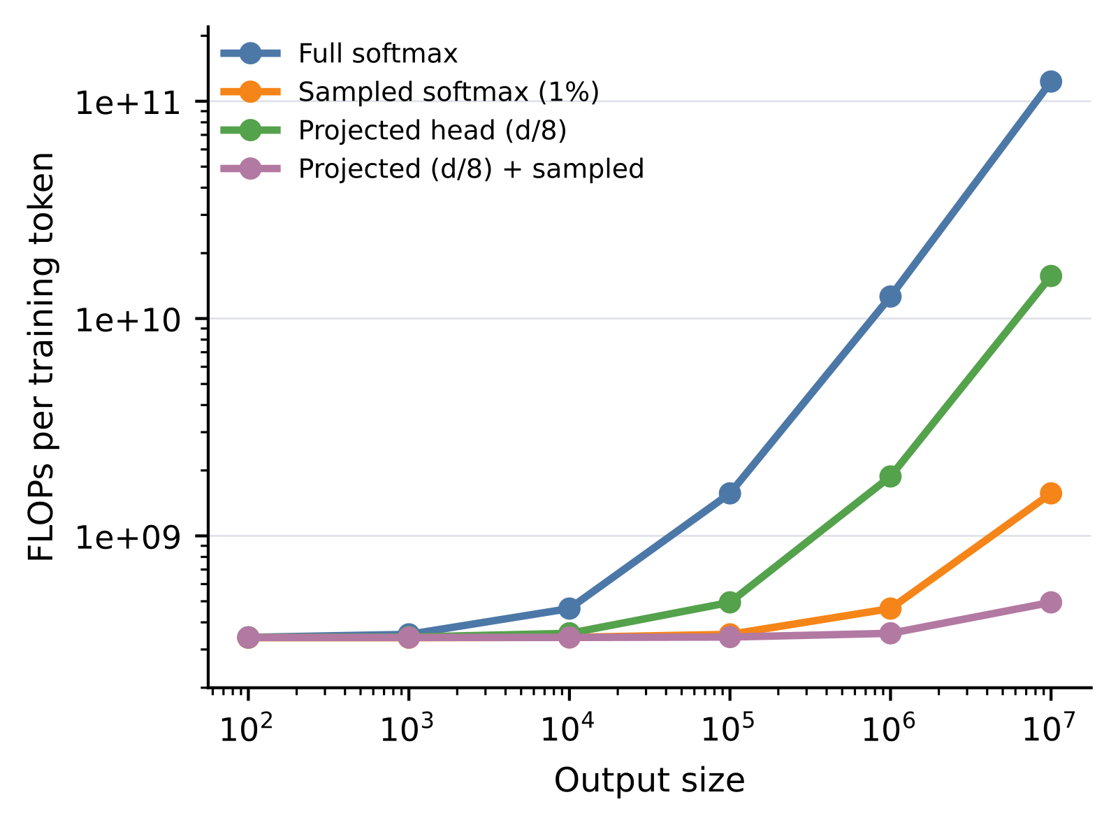
They use two simple measures. First, sampled softmax: during training, logits are computed only for positives and a uniformly sampled 1% of negatives, with any sampled negative equal to the target rejected, and no LogQ correction. Second, a shared projected decoding head: before computing item logits, the backbone hidden state is projected from d to d/8 dimensions, which in production is from 4096 to 512. Backbone capacity is unchanged; only the computation tied to catalog size is compressed.
As an example, with an output vocabulary of 10⁶, the illustrative configuration needs 1.26×10¹⁰ FLOPs per token with full decoding and 3.56×10⁸ FLOPs per token with both measures, which the authors compute as about a 35.5× reduction; at 10⁷ it is about 249×. Note these are analytical output-layer estimates, not measured end-to-end training throughput. The authors also mention a small-to-large experiment funnel: changes are validated first on small backbones and scaled-down test sets, and only those that pass enter 1B training. This is not a method contribution in itself, but it is very practical for controlling the cost of trial and error.
Labels go stale under cached serving: multi-token prediction (MTP)
Seen through the scenario, the cached result is used after the user has finished episode 4, yet next-token training puts all probability mass on episode 4. The authors quantify this with replayed evaluation: as serving delay grows, Task A's MRR changes by at most 4%, Task B drops 31% at a 24-hour delay and 41% at 48 hours, and Task C drops 18% at 48 hours. This shows short-horizon tasks are the most sensitive to cache delay, while long-horizon taste tasks tolerate stale representations better.
The second problem is that many recommendation targets are sets by nature. A user may watch both A and B next, and A-then-B and B-then-A are both reasonable, but next-token training only accepts the one observed order and penalizes other equally valid futures.
MTP builds a weighted set of future targets for each context, containing only high-value future actions, with exponential time decay and a one-hour half-life:
can encode reward signals such as watch time, completion and freshness, and is one hour. The key point is that MTP only changes the supervision target: at serving time the model still scores once, with no step-by-step generation and no extra model calls.
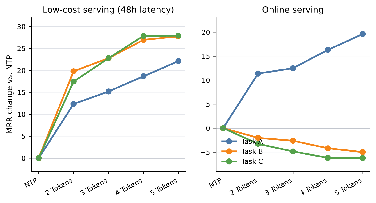
The results split by serving mode. Under 48-hour cached serving, a five-token window is best, with relative MRR gains of 22.1%, 27.8% and 27.9% for Tasks A, B and C. Under online serving with p95 latency below one second, Task A gains 19.6% with five tokens, but Tasks B and C decline as the window grows. This shows MTP suits cached serving and set-like targets, and should be applied cautiously to strict online short-horizon tasks: online, the next event is still a strong target, and widening the target set smooths away the time-sensitive information Tasks B and C rely on most.
Cold start: semantic towers plus ID masking
A new title has no viewing history, so no collaborative ID embedding can be learned, and a bigger model cannot help with that. The authors keep ID embeddings for mature titles and add a multimodal semantic representation for every title, from three sources: graph features from message passing over the title knowledge graph, text embeddings produced with LLM2Vec, and human annotation features.
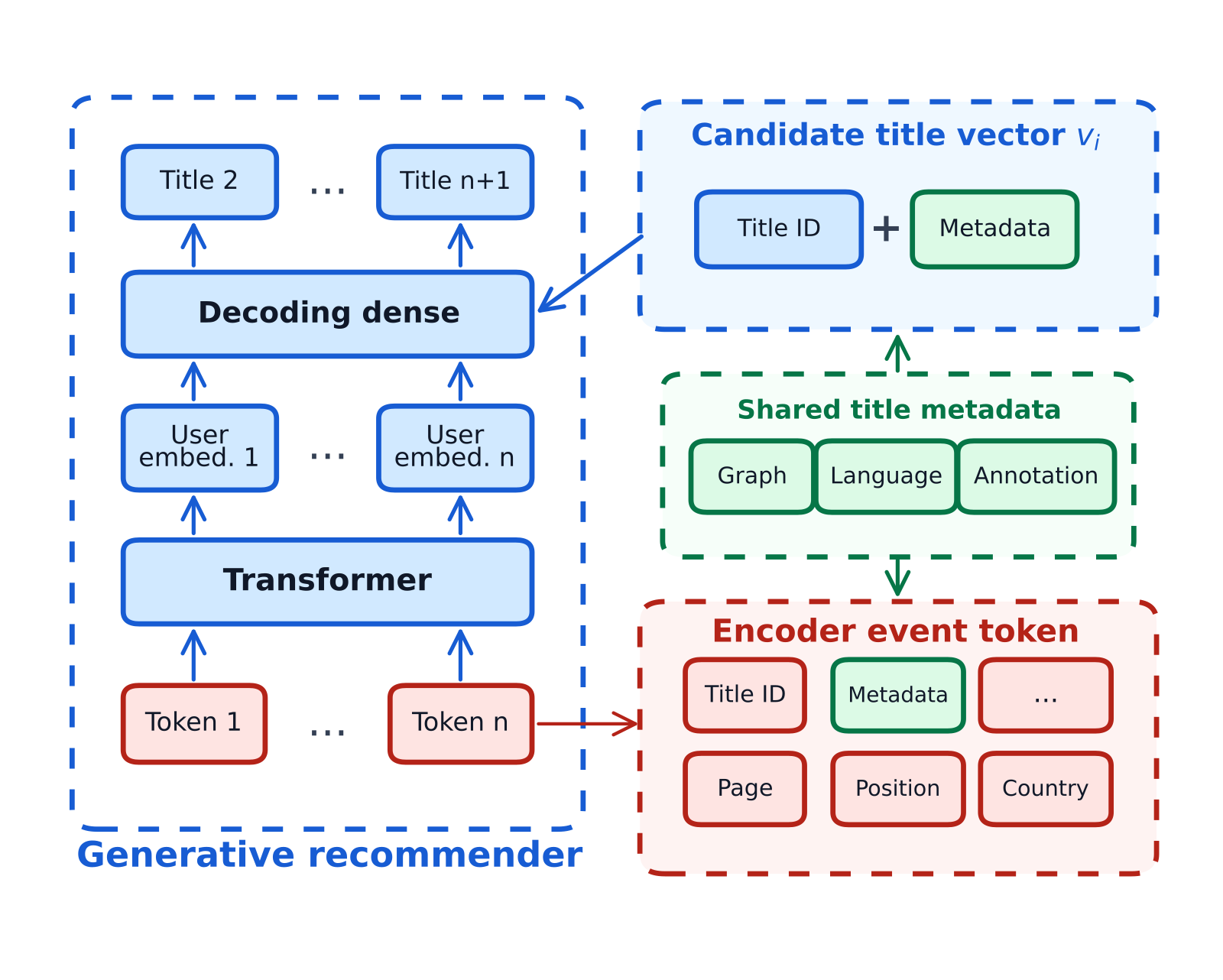
Scoring a title takes three steps: first a mapping combines the graph, text and annotation features into a semantic representation ; then a learned function combines the ID-side embedding and into a candidate title vector ; finally the Transformer's user representation goes through a projection , and its inner product with gives the score . The paper describes only as a learned function; its form (addition, concatenation followed by projection, or another network) is left open. For in-vocabulary titles, the ID side uses the title's own ID embedding; out-of-vocabulary new titles all share one learned OOV embedding, so title-specific information can come only from . To teach the decoder to rely on the semantic representation when ID is missing, pre-training randomly replaces the input-side or output-side collaborative embedding with the OOV embedding, at a rate aligned with the measured online cold-start rate. The new series launched that day in the scenario takes exactly this path: with no ID evidence, it is scored on genre, synopsis and human annotation. Context such as page, position and country only affects the user representation and never enters the candidate title vector, so transient serving context does not leak into the title's own representation.
Production-shadow results
The final comparison is at the production-system level, not a scale-only ablation. The two sides differ as follows:
| Dimension | Baseline | Scaled model |
|---|---|---|
| Backbone | 2M parameters | 1B parameters |
| Decoding | Full softmax | Sampled softmax + projected head |
| Objective | NTP | MTP |
| Cold start | ID embeddings only | Semantic towers + ID masking |
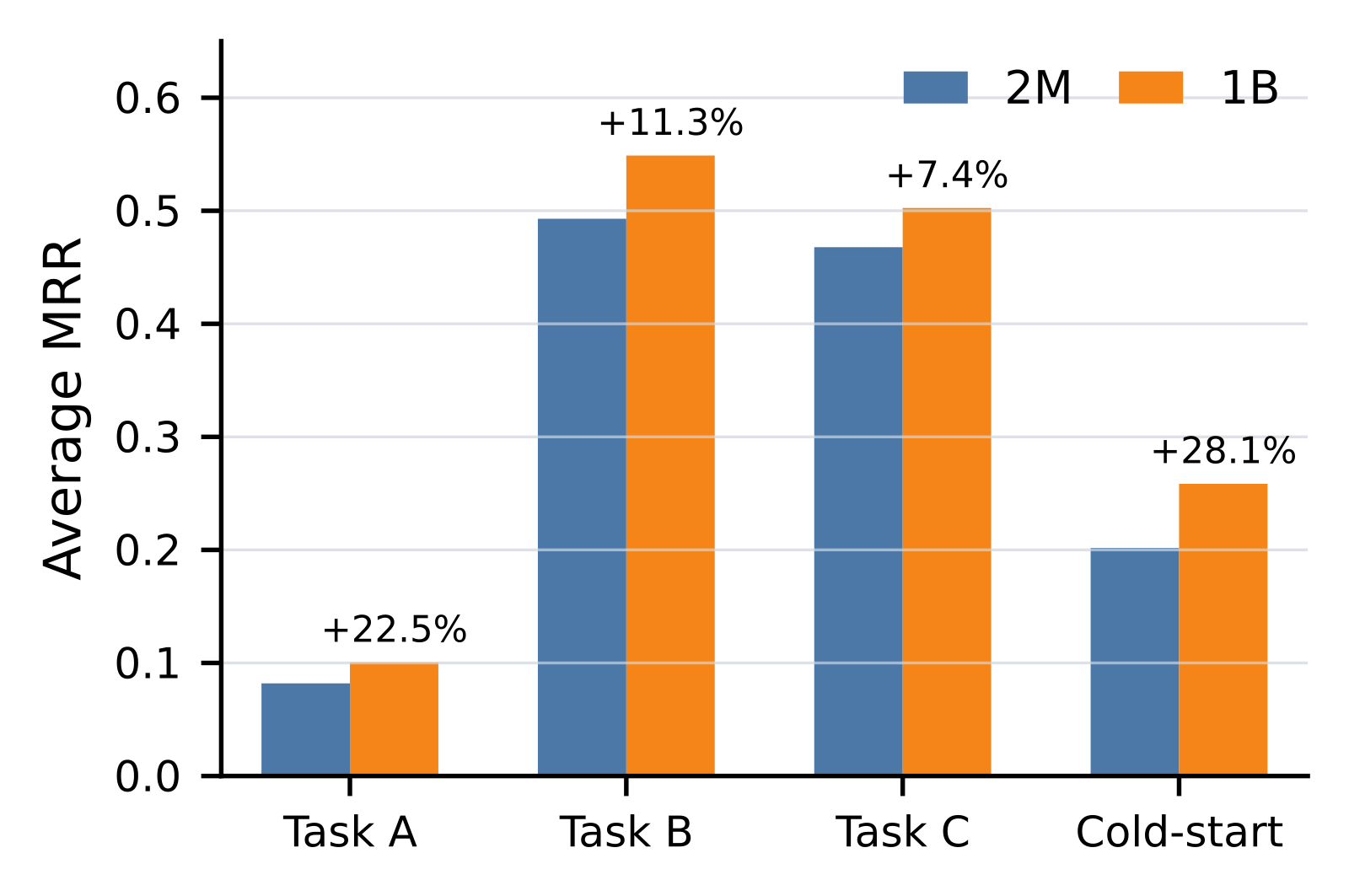
The evaluation covers 1M users over one week. Downstream systems call the model through the production integration path, but the results do not affect what users see, and same-window real behavior serves as labels. The 1B model is better on all four slices: Task A +22.5%, Task B +11.3%, Task C +7.4%, cold-start titles +28.1%. The authors also mention that downstream integrations of the model have produced positive results in multiple online A/B tests, but give no numbers. This shows the combination works across several Netflix downstream scenarios, but this experiment cannot say how much each change contributes.
Limitations as I see them
First, the shadow comparison mixes four variables. Backbone, decoding, objective and cold-start scheme all changed at once, so the 22.5% and 28.1% cannot be credited to "scaling the backbone". The 28.1% cold-start gain especially: the baseline has no semantic tower at all and can only rely on ID embeddings for new titles, so much of the gain may come from the semantic tower rather than the 1B backbone. The authors call the variation in gains across tasks "consistent" with the scaling law, but Task C's fitted headroom is not smaller than Task B's, yet in this comparison Task C gains only 7.4%; together with the confounding, that consistency is hard to check.
Second, the scaling-law evidence is thin. Each task has roughly a dozen points, with no confidence intervals and no held-out larger-scale points to test extrapolation. The offset power law has three parameters and the log-linear form two, so lower fit error on the same points is to be expected; Table 2 is not enough to show it extrapolates better. Task C's of 1.075 exceeds MRR's physical maximum, a reminder that the ceiling estimate carries sizeable error.
Third, several key settings are left unexplained. MTP uses a one-hour half-life, yet it works best in the 48-hour cached setting, and how the weights play out over such a long span is left unexplained; window size is counted in future targets, but which actions count as high-value targets and how long a span those targets usually cover are not spelled out. The cold-start masking rate is only said to match the online cold-start rate, with no value given and no masked-versus-unmasked comparison. The efficiency section is entirely analytical estimates, and uniform negative sampling without LogQ correction may bias scores for popular items, which the paper does not measure.
How a recommendation team could try it
- Start with a per-task scaling diagnosis: take backbones at 3 to 4 sizes, fit ceiling curves per task on fixed data and evaluation sets, and hold out the largest-scale point to test extrapolation. For tasks already near their ceiling, shift resources to the objective and serving path.
- If recommendation results are cached, first run a delay replay: shift evaluation labels forward by 6, 24 and 48 hours and see how much each task drops. Try MTP on the tasks that drop most, sweeping windows from 2 to 5 future targets, and keep NTP for short-horizon tasks served online.
- When cold start is a pressing problem, add semantic towers with ID masking to the existing model and measure new-item performance on its own, without waiting for a backbone scale-up.
- When the output layer dominates training cost, sampled softmax plus a projected head is the cheapest step, but measure real throughput and compare popular and long-tail items with and without LogQ correction.
Conclusion and assessment
The key takeaway: after scaling up a generative recommender's backbone, gains must be read per task, and the bottleneck is often the training objective, serving path and item representation rather than parameter count.
| Dimension | Assessment |
|---|---|
| Problem importance | High. How to land generative recommenders at industrial scale is a problem many teams face now |
| Method novelty | Medium-low. Sampled softmax, multi-token prediction and semantic cold start all have precedents; the contribution is mainly the combination and production experience |
| Experimental evidence | Medium-low. Few scaling-fit points and no confidence intervals; the final comparison mixes four variables, and the A/B tests have no numbers |
| Engineering cost | High. Retraining on 2 trillion tokens per cycle, a 1B backbone and semantic towers all need large-scale infrastructure |
| Worth trying? | Worth borrowing the diagnostics. Per-task scaling curves and cache-delay replay are cheap and give direct answers |
How did this read for you?
Hoot made a note. Thanks for the feedback.

One tap, no sign-in; tap again to undo. Only anonymous counts are kept, never who you are.
Discussion
Add experiment details, reproduction notes or a different take. Requires a GitHub sign-in.
Loading the discussion…