Contents · 5 sections
1What problem does it actually solve?2Method3Results4Limitations5What to borrowSHARE

The pre-ranking stage of a recommender has to pick a few hundred items out of the thousands returned by retrieval and pass them to the ranker, but it can only be trained on items that were shown: feedback (click or no click) exists only when the user saw the item. Online, though, it must score every retrieved item, most of which were never shown. Because training and serving see different data, the model drifts towards popular items and long-tail items struggle to surface. This Alibaba paper proposes GPL (Generative Pseudo-Labeling): offline, a small large language model guesses from a user's history a set of items they might like next; each unshown candidate is compared with these items by content similarity to get a "pseudo-label" between 0 and 1, which is used together with real clicks to train the pre-ranker. In a two-week online A/B test on Taobao's homepage "Guess What You Like" feed, click-through rate rose 3.07% and purchase conversion 2.51%; the share of exposure going to the top 10 categories fell from 70.80% to 45.91%.
It is worth reading for teams working on pre-ranking in cascaded recommenders, or anyone stuck with "we can only train on shown items". The whole pseudo-labelling pipeline runs offline; the online pre-ranker keeps its structure and gains no latency, so the migration cost is mostly offline compute. The evidence comes from one Taobao surface and one public dataset.
What problem does it actually solve?
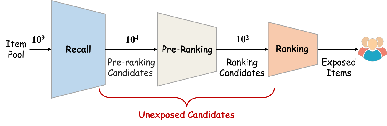
Existing fixes each have problems: treating all unshown items as negatives mislabels items the user would actually like; randomly showing users items to collect unbiased feedback is too expensive; using ranker scores as soft labels for the pre-ranker passes on the ranker's own bias, since it too is trained only on shown items; and adversarial distribution alignment is unstable. The authors' idea is to make pseudo-labels depend only on item content, not on exposure logs, so the bias in behaviour logs is not carried in.
Method
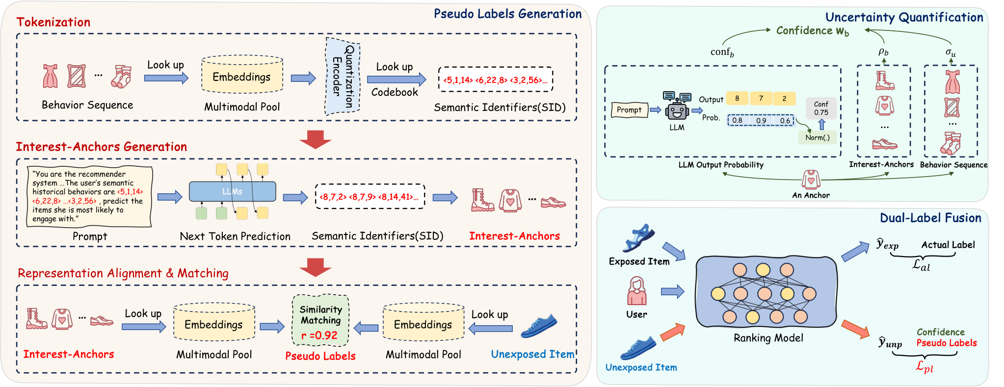
The first step gives every item a code. A frozen multimodal encoder (CLIP on the industrial data) turns an item's image and text into a vector, and residual quantization turns the vector into a short sequence of codes: find the closest vector in the first-level table and record its index, subtract it, and keep looking in the next level. The industrial setup uses 3 levels with 8,192 codes each. Codes depend only on content, so they carry no exposure bias.
The second step guesses interests. The items a user clicked or bought are put in time order and each is replaced by its code; Qwen2.5-0.5B is fine-tuned with LoRA to predict the next item's code. To reduce the weight of popular items, the 10% most frequent items are down-sampled in inverse proportion to their frequency during training. At inference, beam search generates B=32 codes at once, which are looked up to recover real items; more than 98.5% of generated codes are found in the table, and those that are not fall back to the nearest item in the multimodal vector space. These 32 items are the model's guess of "what this user is likely to be interested in next"; the paper calls them interest anchors.
The third step assigns pseudo-labels. For each unshown candidate, compute its cosine similarity with each of the 32 items, take the largest, divide by a temperature and pass it through a sigmoid to get a pseudo-label between 0 and 1. The maximum is used rather than the mean because a few of the model's guesses are always off, and averaging would dilute the one item that really matters.
The fourth step weights by reliability. How trustworthy the model's guesses are this time is measured by three signals:
| Signal | How it is computed | What it tells you |
|---|---|---|
| Dispersion | Mean pairwise cosine distance among the 32 guessed items | The more scattered, the less sure the model is of this user's intent; all of this user's pseudo-labels are down-weighted |
| Consistency with history | Mean similarity between a guessed item and the user's past items | The more it resembles past interests, the more likely it is a real preference |
| Generation probability | Mean log-probability of the code levels when generating that code | Low probability means the model is guessing outside its training distribution |
Concretely: each guessed item first gets a raw score equal to exp(λ₁ × consistency) times exp(λ₂ × generation probability), where λ₁ and λ₂ are tunable coefficients; the 32 raw scores go through one softmax to give relative weights; finally all weights are multiplied by exp(−dispersion), so more scattered users get smaller weights across the board. A candidate's weight is the weight of the guessed item it most resembles. The final loss is cross-entropy on real labels plus λ times weighted cross-entropy on pseudo-labels.
The large model is called per user: each user is generated once a day, independent of how many unshown candidates they have; 96 H20 GPUs finish a day's users in six hours.
Results
The industrial data is 14 days of Taobao logs, about 200 million users, 20 million items and 30 billion interactions; the first 13 days train and the last day validates. Selected results on the industrial data:
| Method | HR@3 | HR@10 | AUC | GAUC |
|---|---|---|---|---|
| Shown items only | 0.4863 | 0.7611 | 0.7096 | 0.6098 |
| Ranker scores as soft labels | 0.4938 | 0.8181 | 0.7110 | 0.6114 |
| Strongest baseline UECF | 0.5216 | 0.8585 | 0.7246 | 0.6313 |
| GPL | 0.5254 | 0.8680 | 0.7299 | 0.6338 |
The gain over the strongest baseline is small (AUC +0.005), but the public dataset Taobao-MM (8.8 million users) points the same way, with AUC going from 0.7055 to 0.7112.
The two most striking ablations: removing real labels and using only pseudo-labels drops HR@3 from 0.5254 to 0.3687, so pseudo-labels can only supplement; removing reliability weighting drops HR@3 to 0.5215. A bigger language model helps, but not much: 7B reaches AUC 0.7354 against 0.7299 for 0.5B, while 7B costs about 17 times more compute per token, so the authors chose 0.5B.
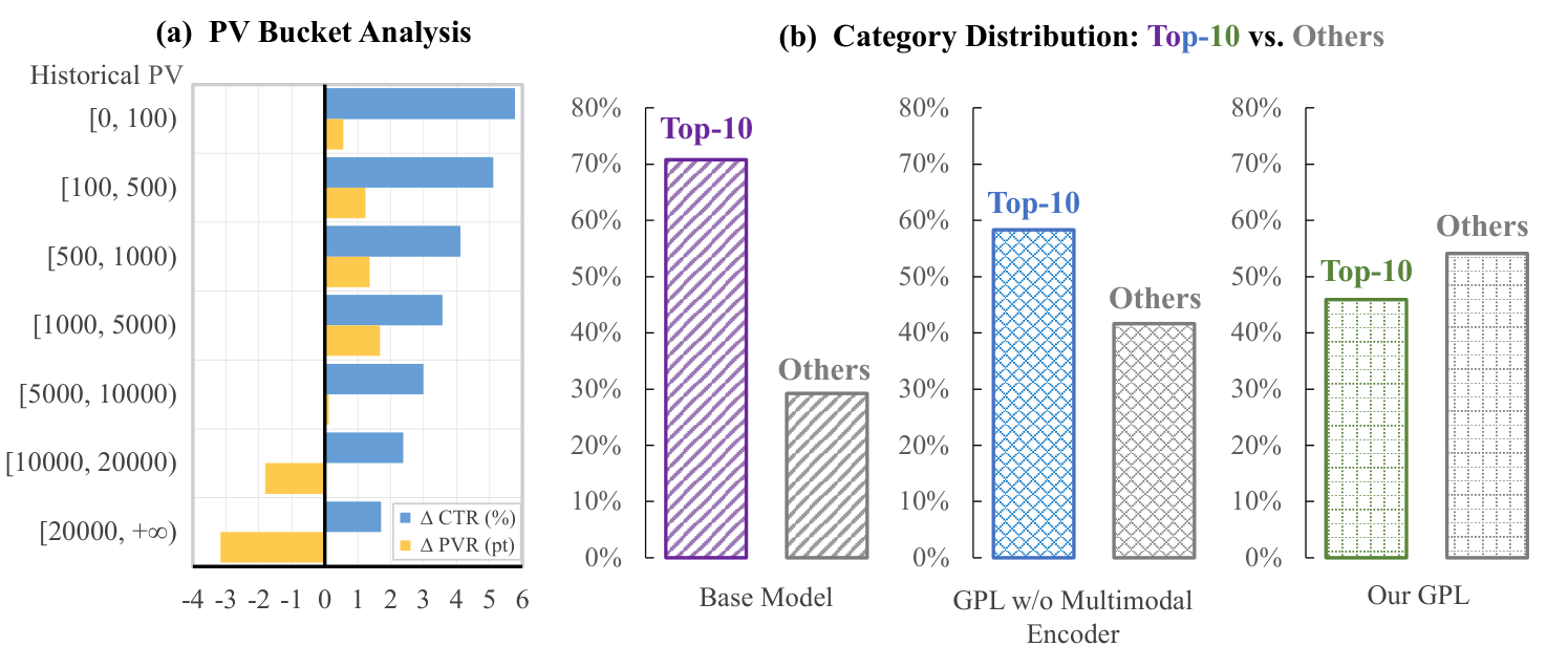
The two-week online A/B test with hundreds of millions of daily users shows item page views +3.53%, click-through rate +3.07%, post-click purchases +2.51%, users who browse more than 200 items in a session +1.50%, and dwell time +2.16%. Bucketing items by historical page views, the colder the item the larger the click-through gain, which shows the pseudo-labels really do surface long-tail items.
Limitations
- Offline cost is not small: every day the large model runs once for every user, and similarity and weights are computed for every unshown candidate.
- Pseudo-label quality is limited: the AUC of pseudo-labels against real clicks is only about 0.63, far below the model itself, so they must be used together with real labels.
- λ and the temperature were chosen by online A/B tests and need retuning in a new setting.
- The offline gain over the strongest baseline is small, and the online gain is measured against the existing pre-ranker, not against those debiasing baselines.
What to borrow
If your pre-ranker has only ever been trained on shown items, the cheapest starting point is: take existing multimodal item vectors, pick a few dozen "possibly interesting" items per user, give unshown candidates a pseudo-label by maximum similarity, add it to the loss with a small weight, and watch whether long-tail click-through improves. The interest-guessing step can start without a large model, using existing retrieval results instead, and be swapped in once the pseudo-label direction is shown to work. Within the reliability weights, "how scattered the guessed items are" is the easiest to implement, and in the ablation it was also the most effective of the three.
How did this read for you?
Hoot made a note. Thanks for the feedback.

One tap, no sign-in; tap again to undo. Only anonymous counts are kept, never who you are.
Discussion
Add experiment details, reproduction notes or a different take. Requires a GitHub sign-in.
Loading the discussion…