SHARE

Mixture-of-experts (MoE) models activate only a few experts per token, so compute is cheap, but every expert's parameters must stay in GPU memory, and memory is usually the first thing that blocks deployment. This paper proposes GS-MoE, which needs no retraining and compresses experts along two axes at once: similar experts are grouped and share one input and one output projection per group, with each expert keeping only a small private matrix; and inside each expert, unimportant intermediate neurons are removed, with the kept neurons used to approximate what the removed ones contributed. On DeepSeek-MoE-16B with 60% of parameters removed, average accuracy on 7 reasoning tasks stays at about 90% of the original model, versus 73% for the baseline D2-MoE.
Teams deploying fine-grained MoE models (many small experts, such as the DeepSeek and Qwen2 MoE models) on memory-constrained machines should look at this. It needs one forward pass to collect statistics and one GPU to compress, and the code is public, so the cost is low. Two caveats: it does not win on Mixtral, which has few large experts; and the paper's own breakdown shows most of the gain comes from the neuron-removal half, while the group-sharing half adds little in most settings.
What problem does it solve?
An MoE model replaces a feed-forward layer with dozens of parallel experts, and a router picks a few for each token. DeepSeek-MoE-16B has 64 experts per layer and uses 6 per token. Compute drops, but the other 58 experts must remain in memory because the next token may need them.
Existing compression methods fall into roughly three types. The first removes or merges whole experts, and quality drops quickly as more are removed. The second makes all experts share one low-rank basis, as in MoE-SVD; but with one shared subspace per layer, any direction unique to an expert that falls outside it can never be represented. The third is D2-MoE, which stores one shared base weight plus a compressed difference per expert, again tying the whole layer together. There are also methods that only remove neurons inside experts, which ignore what experts have in common, so each expert still stores its own weights.
The authors' starting point: similarity among experts is not layer-wide but local, with some experts resembling each other. So experts should first be grouped, share within the group, use different subspaces across groups, and have their internal redundancy compressed too.
Method: group sharing plus neuron removal
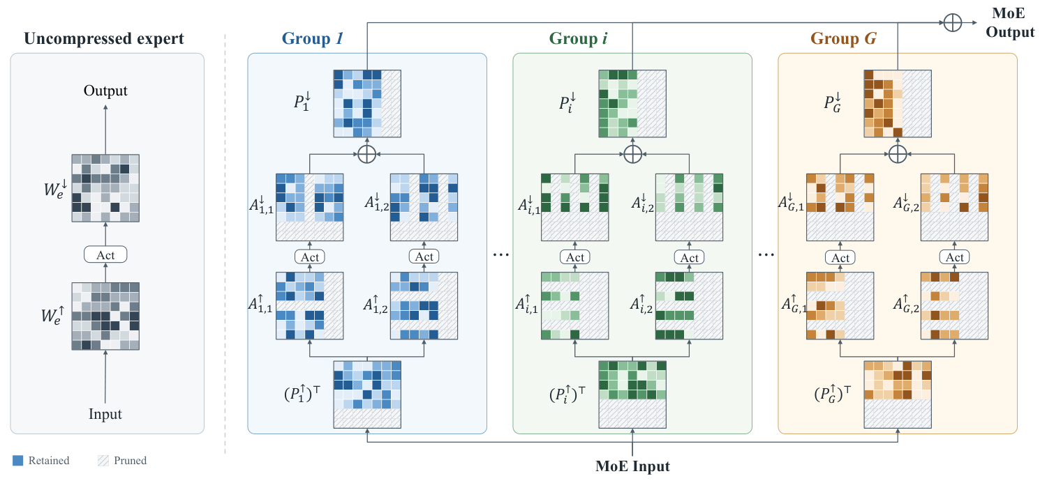
After compression an expert computes in four steps: the input is multiplied by the group's shared input projection into a lower dimension. Then it is multiplied by the expert's own small matrix to get the kept intermediate activations. After the activation function, the expert's other small matrix maps it back to the low dimension. Finally it is multiplied by the group's shared output projection back to the model dimension. Memory savings come from two places: shared projections are stored once per group, and private matrices are small because both sides shrink.
There are four stages.
First, neuron selection. The authors run calibration data through the original model, record statistics of each expert's intermediate activations, and score each neuron with a ridge leverage score that measures how irreplaceable it is: a neuron whose activation is well represented by a combination of other neurons scores low and can be removed. All neurons of all experts in a layer are ranked together and the top K are kept, so different experts keep different widths. K is set by the overall budget, described in the fourth stage.
Second, fitting projections. The output side has a closed-form solution: sum the output covariances of the experts in the group, and the leading eigenvectors form the shared output projection. The input side has none, because experts see different input distributions. The authors average the group's input covariances, weighted by the number of tokens routed to each expert, and treat that as the group's input distribution. The goal is that after the low-dimensional projection, each expert's pre-activation values for its kept neurons can still be reconstructed. Under the averaged distribution this has an approximate solution. For each expert, take the kept rows of its up projection and compute their transpose times themselves, a model-dimension square matrix (so different kept widths do not change its size). Sum these with token weights, multiply on both sides by the square root of the averaged input covariance, take the leading eigenvectors, multiply by the inverse square root and orthonormalize. With the shared projection fixed, each expert's private matrix is a least-squares fit on that expert's own input covariance. Removed neurons are compensated with the Nyström approximation, a classic method for reconstructing a full covariance matrix from a few kept columns: from the recorded intermediate-activation covariance, compute a linear map that predicts the full intermediate activation from the kept neurons, and fold that map into the private down matrix. The down projection then reads only kept neurons yet approximates the contribution of all of them.
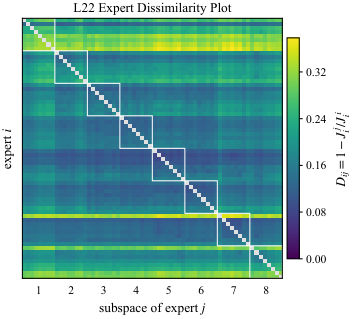
Third, grouping. The authors derive a score for how much an expert's reconstruction error drops inside a candidate subspace. They fit a subspace for each expert alone, then put expert i into expert j's subspace, reconstruct expert i's kept pre-activations and outputs, add the two errors (the output term is scaled by the fraction of up-projection output energy retained after neuron removal, to balance the two terms), and measure the drop from the no-reconstruction error. Dividing by the drop expert i gets in its own subspace gives a ratio; one minus it is the dissimilarity. With a 64×64 dissimilarity matrix, balanced clustering produces equal-size groups.
Fourth, capacity allocation. Each layer gets an importance score: for each token routed to an expert, the expert's output norm times the routing weight divided by the input norm, averaged over that expert's tokens and summed over the layer's experts. The target compression ratio gives the overall retained fraction R of expert parameters; a hyperparameter ν (0.45 to 0.55 by default) sets the width retention to R to the power ν, and the shared-dimension retention follows as R divided by the width retention plus the shared-projection overhead. Removal is spread across layers by a softmax over negative log importance, so less important layers lose more. Within a layer, eigenvalue sums decide each group's shared dimension under the layer budget.
The whole process takes one forward pass over 512 Alpaca samples of 2048 tokens each, fits on one GPU, and involves no training afterward.
Does grouping actually help?
The authors ablated this on DeepSeek-MoE-16B at 60% compression using only group sharing, without neuron removal. Without grouping, WikiText-2 perplexity is 29.49; with score-based grouping it falls to 25.23, because similar experts lose less when sharing a subspace. Adding per-group dimension allocation lowers it a further 0.57 on average across three datasets. Without grouping, dimension allocation alone brings no consistent gain.
Grouping has a side benefit: if a token's selected experts fall in the same group, the shared projection is computed once. With 8 groups each token touches only 3.68 groups on average, about 19% fewer than random grouping.
Results
The authors compare against MoE-SVD, D2-MoE, TD-MoE and others on three models, using average accuracy over 7 zero-shot reasoning tasks and perplexity on WikiText-2 and PTB (another language-modeling test set). Compression ratio is the reduction in total model parameters.
| Model and ratio | Original | D2-MoE | GS-MoE |
|---|---|---|---|
| DeepSeek-MoE-16B, 40% | 0.56 | 0.49 | 0.54 |
| DeepSeek-MoE-16B, 60% | 0.56 | 0.41 | 0.50 |
| Qwen2-57B-A14B, 40% | 0.59 | 0.58 | 0.59 |
| Mixtral-8x7B, 40% | 0.63 | 0.57 | 0.57 |
| Mixtral-8x7B, 60% | 0.63 | 0.52 | 0.50 |
On the two fine-grained models GS-MoE leads clearly: 0.50 versus 0.41 on DeepSeek at 60%; Qwen2 at 60% still averages 0.59, equal to the original, while the next best, TD-MoE, reaches 0.52. On Mixtral, with only 8 large experts, it ties D2-MoE and is slightly worse at 60%, which suggests the advantage comes from many fine-grained experts.
Perplexity is more mixed. On DeepSeek at 60%, GS-MoE scores 22.21 on PTB versus 27.73 for D2-MoE, 20% lower, which is the source of the abstract's out-of-domain claim; but on WikiText-2 it scores 17.55, clearly worse than D2-MoE's 11.67. Which method is better depends on the metric you look at.
On speed, 60%-compressed Mixtral on a B200 runs at 374.77 tokens per second with GS-MoE without grouping, 3.32 times D2-MoE, because D2-MoE must reconstruct residuals for every expert. Going from 1 to 8 groups lowers DeepSeek throughput by only 9.6%.
Limitations as I see them
First, the two halves contribute unevenly. The appendix tests group sharing only and neuron removal only: on Qwen2 and Mixtral, neuron removal alone is nearly as good as the full method; only on DeepSeek at 60% is the full method clearly better (0.503 versus 0.487). In many settings, Nyström neuron removal alone gets most of the gain.
Second, it does not suit models with few large experts. The authors acknowledge that Mixtral's large intermediate size and 8 experts make lowering the subspace dimension more damaging and leave little to group.
Third, evaluation covers only language modeling and multiple-choice reasoning, with no generation, long context or code, and no combination with quantization. In practice MoE deployments more often quantize or offload rarely used experts to CPU memory; the paper does not compare against those.
How a team could try it
- Confirm your model is a fine-grained MoE with around 64 experts or more.
- Run only the neuron-removal part first and measure the loss at 40% compression on your own evaluation set; it is the cheapest step.
- To reach around 60%, add group sharing and check generation quality, not just perplexity.
- Increase the number of groups gradually and measure throughput at each step, since more groups mean more shared projections and slightly lower speed.
Bottom line
Experts in fine-grained MoE models are locally similar; grouping them to share subspaces and then removing redundant neurons cuts 60% of parameters without training while keeping most reasoning ability, but most of the gain comes from neuron removal and it does not win on models with few experts.
| Dimension | Assessment |
|---|---|
| Problem importance | Medium-high. MoE memory footprint directly blocks deployment |
| Novelty | Medium. The grouping score and capacity allocation are new; the components are existing tools |
| Evidence | Medium. Three models, several ratios, ablations and throughput; perplexity and accuracy disagree; no generation tasks |
| Engineering cost | Low. No training, one forward pass, one GPU, public code |
| Worth trying | Yes for teams deploying fine-grained MoE under memory limits; start with neuron removal |
How did this read for you?
Hoot made a note. Thanks for the feedback.

One tap, no sign-in; tap again to undo. Only anonymous counts are kept, never who you are.
Discussion
Add experiment details, reproduction notes or a different take. Requires a GitHub sign-in.
Loading the discussion…