 RecSys 2026
SHARE

Search ads on local-services and live-commerce platforms have a structural mismatch: the platform ranks and charges per store or per livestream room, but the user actually pays for one voucher or product inside it. A user taps into a dental clinic, the model scores it high because "this store converts to a lot of money", and the merchant pays a premium for the click; then the user buys only a cheap teeth-cleaning voucher instead of an implant, and the merchant loses money on that ad. This Meituan paper (RecSys 2026) estimates a store's expected transaction value by splitting it apart: first estimate whether the user buys anything in the store, then estimate the purchase probability and quantity of each voucher, multiply by the voucher price and sum. Once it is split, every sub-task has a far more stable label, and the model is no longer dragged around by the occasional big order. In a 13-day online A/B test, ad revenue per search rose 1.42%, and the method is now serving all main traffic.
Teams ranking ads for e-commerce, local services or live commerce should read it. The paper is only four pages and the modules are not new, but it states a common and rarely isolated problem clearly: when the unit you rank differs from the unit that transacts, regressing "how much money did this click produce" directly barely learns. The core idea in one sentence: a store-level model decides "will the user buy", voucher-level models decide "which voucher and how many", and a general regression tower backs up the samples whose voucher-level signal is too sparse. Offline ranking quality (XAUC) rises from 0.8105 for the strongest baseline to 0.8158, and the ratio of predicted to actual transaction value goes from about 0.79 to 0.9858, i.e. essentially calibrated.
What problem is it really solving?
Walk through the scenario first. A user searches "teeth cleaning" in a local-services app and gets ads for two dental clinics. The platform ranks and charges them by something like "expected post-click transaction value × click-through rate", so every store needs an estimate of its expected post-click transaction value (the paper calls it GTV, gross transaction value).
| Store (illustrative) | Vouchers in the store | Actual transactions after 100 clicks in a week |
|---|---|---|
| Clinic A | Cleaning 153 yuan, air-polish cleaning 418 yuan, implant 6000 yuan | 95 no purchase; 4 cleanings; 1 implant |
| Clinic B | Cleaning 99 yuan, whitening 800 yuan | 92 no purchase; 8 cleanings |
If you regress directly on "how much did this click transact", Clinic A's labels are almost all 0, occasionally 153, and very rarely 6000. That one implant pulls the store's average transaction value up to about 66 yuan, yet it may well be luck; next week nobody buys an implant and the average falls to 6 yuan. Because the gradient is dominated by a handful of big orders, the ranking a model learns from such labels is very unstable.
The paper names three difficulties, and they map directly onto the table:
First, high label variance. In the same premium store a user may buy only the cheapest voucher out of a passing preference, so the value of a single click does not represent the store's real value.
Second, extremely sparse voucher-level labels. Store-level purchases are already far sparser than clicks; purchases of one specific voucher are rarer still, so modeling directly at the voucher level has almost no supervision.
Third, a store is a changing set of vouchers. Each store lists different vouchers, prices and discounts, which come and go, and the model has to learn the relation between "this user, this query, this store" and "this particular set of vouchers" jointly.

The usual shortcut is to treat the store as a "super item": multiply an average order value by the store's conversion rate, or predict the conversion of the most popular voucher only. The paper's criticism is direct: neither sees which vouchers the store has or which one the user will buy, so stores with many expensive vouchers get undervalued and stores with many cheap ones get overvalued.
Overall structure: three components, one job each
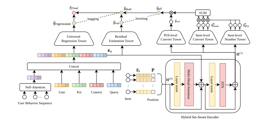
The paper calls the whole method HGE (Hierarchical GTV Estimation). Data flows bottom-up:
| Stage | Input | Output |
|---|---|---|
| Set encoder | The store's 10 most-displayed vouchers + user, store, context and query features | A context-aware representation per voucher |
| Decomposed estimate | Voucher representations | Store purchase probability × Σ(voucher purchase probability × quantity × unit price) |
| Residual correction | User, store, context and query features | Covers purchases outside the top 10 vouchers |
| Weighted blend | Corrected decomposed estimate + general regression tower estimate | Final expected post-click transaction value |
The key division of labor: the decomposition turns one hard-to-learn large number into several easy-to-learn small numbers, while the residual and blending keep the decomposed result from drifting when voucher-level signal is weak. Let's take them one at a time.
The set encoder: why not just average the vouchers?
The paper calls this step HSAE (Hybrid Set-Aware Encoder). It answers this question: the same set of vouchers in the same store is worth different amounts to different users and queries. A user searching "teeth cleaning" rarely buys the implant voucher however expensive it is; for a user searching "implant price", the cleaning voucher is just filler. Averaging all voucher embeddings erases that difference.
Concretely, it first takes each store's 10 most-displayed vouchers and adds a position embedding to each voucher embedding so the model knows the order in which vouchers are shown. It then runs one layer of Transformer multi-head self-attention so vouchers can see each other and learn "is this the cheap one or the expensive one in this set". Finally, after the attention layer and before the FFN, it concatenates the user, store, context and query features.
Why inject those features only after attention? The paper's reason is a trade-off: inject too early and the voucher-to-voucher comparison is diluted by many external features; leave them out and the same set of vouchers gets one representation for every "user × store × query" combination. Letting vouchers compare within the set first and then modulating with external features handles both. It is a small detail but a practical one: teams doing set modeling often agonize over which layer the user features should enter.
The decomposition: split one big number into three small ones
This is the most important component, which the paper calls PLL (Proxy-Label Learning). "Proxy labels" means not using transaction value directly as the label, but supervising separately with steadier signals: did the user buy, which voucher, and how many. The decomposition is:
is the probability that the user buys any of the store's top vouchers; is the probability of buying voucher given that a purchase happens; is the quantity of that voucher; is the voucher's unit price, taken as known rather than learned. The first two use a sigmoid output in 0 to 1; quantity uses softplus to stay positive. The two voucher-level towers share parameters across vouchers, so newly listed vouchers can be scored immediately.
Work it through for Clinic A (illustrative numbers). Store purchase probability 0.05; given a purchase, the probabilities of buying the cleaning, the air-polish cleaning and the implant are 0.70, 0.25 and 0.05; quantities are 1.2, 1 and 1. Then:
- Cleaning: 0.70 × 1.2 × 153 ≈ 128.5
- Air-polish cleaning: 0.25 × 1 × 418 = 104.5
- Implant: 0.05 × 1 × 6000 = 300
The sum is about 533 yuan; times 0.05, the expected post-click transaction value is about 26.7 yuan. This number stays roughly the same every day because it is set by three smooth quantities — purchase rate, the distribution over vouchers, and quantity — and it does not jump to 66 yuan because someone happened to buy an implant that day.
Why is the split steadier? The paper argues with the law of total variance; the intuition is that regressing transaction value directly asks the model to learn a target that is mostly 0 with an occasional large number. After splitting, purchase-or-not is a 0/1 classification, quantity is at most 2 in over 90% of purchases, and which voucher is a probability distribution, so each sub-task has a narrow output range and far smaller variance. The price, which is what really causes the big variance, is moved onto a known number the model no longer has to learn. The split has a side benefit: the model can tell "expensive but rarely bought" from "cheap but bought by everyone", two kinds of store that direct regression may score the same.
Residual and blending: what if voucher-level signal is too sparse?
The decomposition alone leaves two holes, which the paper fills with a component called RCEF (Residual Correction and Ensemble Fusion).
The first hole is that the top 10 vouchers do not cover everything. A user may buy a voucher ranked 11th or lower in the store, and that purchase never appears in the decomposition. So a lightweight residual tower looks only at user, store, context and query features and outputs a correction that is added to the decomposed estimate.
The second hole is that voucher-level signal is too sparse. In many samples the user has barely interacted with the store's vouchers, and the two voucher-level towers are mostly guessing. A model that regresses transaction value directly at the store level is more reliable there. The paper builds this general regression tower from DIN plus DCN and blends it with the corrected decomposed estimate:
is the decomposed estimate plus the residual correction, and is the general regression tower's estimate. The weight is not fixed: a small gating network computes it per sample from "user × store × context". Think of it as trusting the decomposition more when voucher-level signal is rich and the store-level regression more when it is sparse (illustrative: might be only 0.3 for a new store and reach 0.8 for an established store with frequent orders). Hoot says

Forward: one new-store sample (illustrative)
- top-10 decomposition
- 40 yuan
- + residual tower
- correction +6 (for what the top 10 vouchers miss) → ŷ_deal = 46
- regression tower
- ŷ_regression = 30
- new store α = 0.3
- 0.3 × 46 + 0.7 × 30 = 34.8
- an established store, α = 0.8
- 0.8 × 46 + 0.2 × 30 = 42.8
Same two branches, but a different α moves the result by 8 yuan: the gate decides which branch this sample trusts.
Backward: how the two label-less parts learn
- suppose the true amount
- 40 yuan; the new-store estimate is 5.2 short
- to the residual tower
- ∂ŷ_final / ∂residual = α, so it gets only 0.3 of the gradient
- to the gate
- ∂ŷ_final / ∂α = ŷ_deal − ŷ_regression = 16 > 0 and the estimate is low → this sample's α is pushed up
- if only the regression tower were supervised
- both get no gradient at all
So the regression loss must supervise ŷ_final; in sparse new stores the residual tower already learns slowly.
All amounts are illustrative, not from the paper; α of 0.3 and 0.8 follow the text's illustration. The gradient directions on the right come from differentiating the blend formula; the paper does not show this step, and "the regression loss supervises ŷ_final" is likewise inferred from the formula. Source: paper, RCEF: a residual tower (user, store, context, query features) corrects the top-10-voucher decomposition; a DIN + DCN general regression tower; ŷ_final = α·ŷ_deal + (1 − α)·ŷ_regression with a per-sample gate α; four tasks trained jointly
Training learns four tasks jointly: general regression and quantity use Huber loss (squared for small errors, absolute for large ones, which weakens the pull of big orders), and store purchase and voucher purchase use cross-entropy. The weights are 1 for regression, 0.3 for store purchase, and 0.03 each for voucher purchase and quantity. The residual tower and the gating network have no labels of their own. By the formula they can only get gradients from the error between the final estimate and the actual transaction value, so the regression term should supervise the final estimate, not only the general regression tower (this is our reading of the formula's structure).
Experiments: how much does splitting buy?
The offline data comes from Meituan's ad logs: 712 million samples, 121 million users, 949 thousand stores. It is split by time, with the last 5% of samples used for testing so the model never trains on future data. Three metrics: XAUC is the fraction of random sample pairs where the predicted transaction values are ordered the same way as the actual ones, measuring ranking; PCOC (predicted over actual) is total predicted transaction value divided by total actual value, where closer to 1 means better calibration; MAE (mean absolute error) measures how far off each sample's estimate is.
There are four baselines: WLR (rewrites value regression as weighted binary classification, the old trick YouTube used to predict watch time); DLRM (the standard deep regression with DIN for sequences and DCN for feature crossing); RankMixer (a ranking architecture that replaces self-attention with token mixing); and CREAD (turns continuous-value prediction into multi-class classification to improve calibration).
| Method | XAUC | PCOC | MAE |
|---|---|---|---|
| WLR | 0.8043 | 0.7663 | 5.1453 |
| DLRM | 0.8051 | 0.7787 | 5.0453 |
| RankMixer | 0.8105 | 0.7528 | 5.1735 |
| CREAD | 0.8095 | 0.7921 | 5.0818 |
| HGE | 0.8158 | 0.9858 | 4.9915 |
The XAUC gain looks small, 0.0053 above RankMixer. But on a target as noisy as transaction value, the four baselines differ from one another by at most 0.0062, so the margin is not small. Calibration is the clearer story: every baseline's total prediction is only 75% to 79% of the actual value, while HGE reaches 98.6%. Regressing transaction value directly makes the model systematically underestimate, and after splitting that underestimation is essentially gone.
The ablation separates each component's contribution:
| Variant | XAUC | PCOC | MAE |
|---|---|---|---|
| Full model | 0.8158 | 0.9858 | 4.9915 |
| Without set encoder | 0.8031 | 1.1012 | 5.2586 |
| Without decomposition | 0.7873 | 0.4180 | 6.9875 |
| Without residual and blending | 0.8146 | 0.9960 | 5.0130 |
Without the decomposition, XAUC drops to 0.7873, worse than every baseline, and PCOC falls to 0.418, less than half the actual value. Most of the gain comes from splitting the estimate itself. Without the set encoder, XAUC drops by 0.0127 while PCOC overshoots to 1.10: once vouchers are averaged, the model cannot tell which voucher will be bought and tends to overcount expensive vouchers. Without the residual and blending, XAUC drops only 0.0012; its effect is mainly on error, with MAE going from 5.01 down to 4.99.
Online, the authors ran a 13-day A/B test after an A/A phase confirmed the two groups matched. HGE lifted RPS (ad revenue per search) by 1.42%; the lower bound of the 95% confidence interval is 0.80%, which excludes 0, so the lift is significant. On mainstream search-ad traffic, that is enough to justify a full rollout.
Limitations as I see them
First, the evidence for the residual-and-blending component is thin. Removing it costs only 0.0012 XAUC, and PCOC goes from 0.9858 to 0.9960, which is actually closer to 1. The only support is a small MAE improvement. Adding a residual tower and a gating network for that gain looks out of proportion; seeing how the gating weight is distributed across new and established stores would show whether it really switches with signal density.
Second, there is only one in-house dataset, and the baselines' low PCOC may partly reflect calibration. All four baselines have PCOC between 0.75 and 0.79, a systematic underestimate. Production ranking models usually apply a calibration step after the output. If the baselines skipped it, part of the gap from 0.79 to 0.99 comes from calibration rather than from the architecture.
Third, price is treated as a known constant. Voucher prices really are fixed in this setting, but big promotions, flash discounts and spend-and-save offers make the actual paid price differ from the list price. Also, the top 10 vouchers are chosen by display count, a fairly static set; for stores that list and delist vouchers often, the set encoder may be looking at a stale voucher list.
How a recommendation or ads team could try it
- First confirm you have the same mismatch: the ranking unit is a store, livestream room, shop or item bundle, and transactions happen on sub-items inside it. Look at the distribution of post-click transaction value; if more than 90% is 0 and a few are large, it is worth trying.
- Start with the cheapest version: add only the decomposition. Reuse your existing CVR model as the store purchase tower, add a voucher-level purchase tower and a quantity tower, and multiply by the known prices and sum. Offline, check whether PCOC moves clearly closer to 1 without XAUC dropping.
- If that works, add the set encoder. The thing to watch is whether, after dropping average pooling, stores dominated by expensive vouchers and stores dominated by cheap ones get more clearly separated estimates.
- Consider the residual and blending last. First measure the share of purchases outside the sub-item set; if it is small you can skip it for now. In the online A/B, track merchant ROI alongside revenue so platform revenue does not rise while merchants' return gets worse.
One-line conclusion
When the unit you rank differs from the unit that transacts, do not regress transaction value directly: split it, following the user's decision order, into "will they buy, which item, how many", then multiply by the known price. That step alone delivers most of the gain.
| Dimension | Assessment |
|---|---|
| Problem importance | High. Local-services, live-commerce and shop ads all rank stores while sub-items transact |
| Method novelty | Medium. Splitting probabilities in the user's decision order is close to ESMM; what is new is putting the sub-item set and prices explicitly into the split |
| Experimental evidence | Medium. 712 million samples and a significant 13-day A/B, but one in-house dataset and weak ablations for some components |
| Engineering cost | Medium-low. Mostly a few extra towers and a single Transformer layer; price is an existing feature |
| Worth trying | Yes. Ship the decomposition alone first: lowest cost, largest gain |
How did this read for you?
Hoot made a note. Thanks for the feedback.

One tap, no sign-in; tap again to undo. Only anonymous counts are kept, never who you are.
Discussion
Add experiment details, reproduction notes or a different take. Requires a GitHub sign-in.
Loading the discussion…