SHARE

In ad systems, recalibrating a CTR model on the last few hours of fresh data is usually treated as a routine step that can only help. This paper checks it day by day on ten days of Avazu ad logs and finds that a calibrator fitted on the preceding 6 hours makes calibration error worse about a third of the time, in the worst case doubling it. Widening the fitting window to the preceding 12 hours largely removes the harm, and uniformly sampling just 5% of those 12 hours recovers 88% of the full window's calibration improvement. In this control, the number of rows alone does not explain the improvement and the time span matters more; but span also changes which hours of the day are covered, how many distinct hours are sampled and how old the data is, and the author did not separate these.
Teams doing bidding, budget control, or anything else that consumes pCTR values directly should read this, because it points to a failure mode that is rarely checked: the calibration job runs every day as scheduled while quietly making predictions worse, and the damage is hard to notice afterwards. It is, however, a single-author measurement study on one dataset, Avazu from 2014, and the two training origins share most of their test days. The specific "12 hours is best" number cannot be carried over to other logs; what is worth taking away is the measurement method: count, per day, per training origin and per random seed, how often recalibration helps and how often it hurts.
What exactly is being measured?
In an ad system a CTR model's output is not only used for ranking. Expected-value bidding multiplies pCTR by the value of a click; budget control compares predicted against realized click rates to decide whether to release or tighten spend. A model with excellent AUC that overestimates by 10% across the board makes every bid too high. So production systems usually add a calibration layer after the model: take the latest labeled data, fit a monotone map, and correct raw scores toward actual click rates.
The paper tests the two most common calibrators. Platt scaling fits a two-parameter logistic regression on top of the model's score, shifting and stretching it as a whole; isotonic regression is a piecewise-constant monotone map that can correct different score ranges by different amounts, so it is more flexible. Calibration quality is measured by ECE: split predictions into 15 bins, compare each bin's mean prediction with its actual click rate, and average the gaps weighted by bin size.
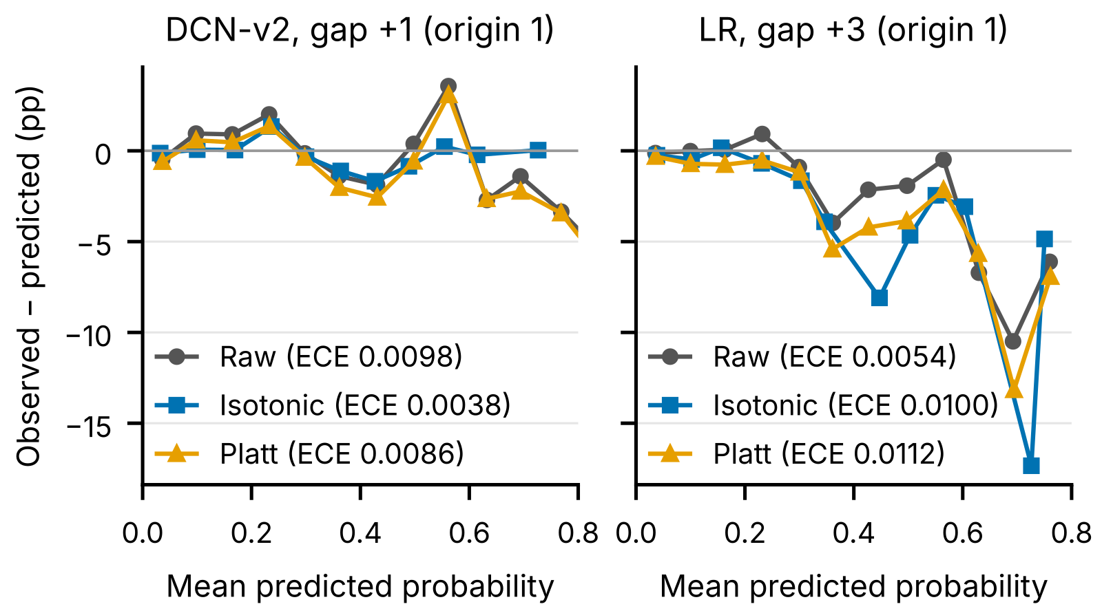
A concrete case shows how harm happens (numbers from one LR cell in the paper's Table I):
| Time | Model's mean bias (predicted minus actual) | What the calibrator does |
|---|---|---|
| Previous day, 18:00 to 24:00 (fitting window) | -0.0071, under-predicting | Learns "push predictions up overall" |
| Next full day (target day) | +0.0031, already over-predicting | Gets pushed up further; ECE rises from 0.0054 to 0.0112 |
The window and the target day are biased in opposite directions. The calibrator faithfully learns the window's pattern and then does damage when applied to the next day.
How the experiment is set up
| Setting | Details |
|---|---|
| Data | Avazu, about 40.43 million impressions, October 21 to 30, 2014, overall click rate 16.98% |
| Models | LR, DeepFM, DCN-v2, each training set capped at 4 million rows |
| Training origins | Origin 1 trains on days 0 to 4 and tests on days 5 to 8; origin 2 shifts everything one day later |
| Control | A random split of the same data |
| Calibration | Each test bucket fits Platt and isotonic on the slice immediately before it: the nearest test day (gap 0) fits on its own first 6 hours and is evaluated on the rest of that day, the other days on the previous day's last 6 hours; a calibrator never sees the data it is scored on or anything after it; the main experiment uses 6 hours, with a sweep over 1, 3, 6, 12 and 24 hours |
| Downstream | A simulated second-price auction bidding by pCTR, comparing profit |
| Replication | Three random seeds |
The main experiment has 2 origins × 4 test days × 3 models × 2 calibrators = 48 calibration applications.
Finding 1: random splits make calibration look too good
In a random split, test and training rows come from the same days, so the model is examined on "time it has already seen". On origin 1's nearest test day, random-split AUC is about 0.014 higher than the temporal split; the ECE gap is larger: LR's random-split ECE is only 55% to 62% of its temporal value, in all three seeds. In other words, if the only pre-launch check is "is ECE below some threshold" on a random split, the quantity being measured is not the one the model will face after launch.
This gap is not stable, though. At origin 2 the AUC gap on the nearest test day almost vanishes, and the two deep models' ECE ratios swing widely across seeds; only LR is stable. The authors therefore rest this conclusion on LR alone, a restrained way to write it.
Finding 2: calibration error does not get steadily worse over time
A common intuition is that the farther a test day is from the training window, the more distribution drift there is, and the higher the ECE. The paper's data does not support this.
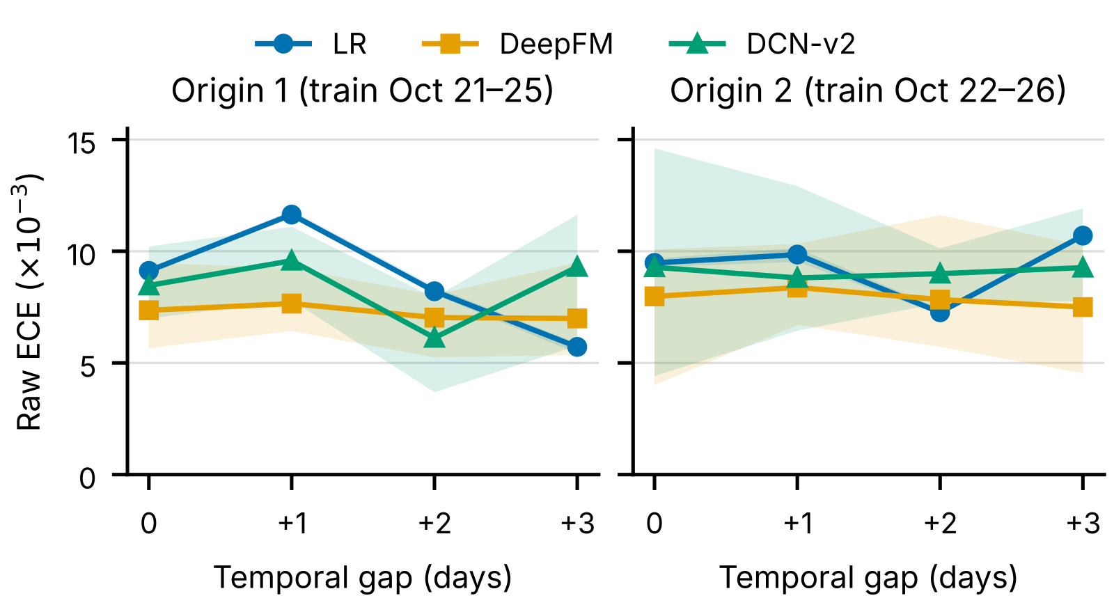
At origin 1, LR is worst on the second test day and then gets better; at origin 2 it is best on the third day and worst on the fourth. The same calendar day also has different ECE under the two origins: LR's ECE on October 28 goes from 0.0082 to 0.0099. Moving the training window by one day changes a given day's calibration about as much as switching to another test day. That means "older models are less accurate" cannot be the only basis for scheduling retraining and recalibration.
Finding 3: with a 6-hour window, one recalibration in three does harm
Of the 48 applications, the three seeds have 16, 14 and 17 that make ECE worse, so "about a third" is not a fluke of one seed. When the raw model is badly off, recalibration often works well, and the best case cuts ECE by 61%; but a high raw ECE does not guarantee recalibration helps, as the figure below has harmful points in the high-ECE region too.
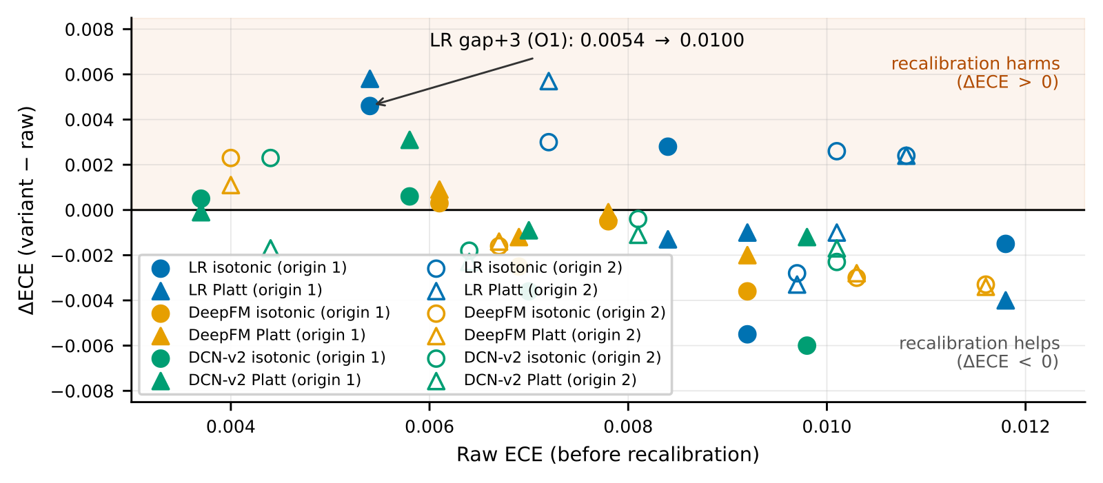
Why does this happen? The author argues that too few samples is unlikely to be the sole cause: a 6-hour window holds 620,000 to 1.01 million impressions, and Platt, with only two parameters, is estimated almost without error, yet it can still double ECE. The author also notes that estimation error in sparse score regions is not ruled out. A better explanation is a mismatch in direction: the fitting window is the previous evening's six hours, while the target is a whole new day with a different mix of hours, traffic and click rate. Two after-the-fact rules check this: "harm happens when the window's and target day's biases have opposite signs" is right on 83% of the 48 applications; "harm happens when subtracting the window's bias from the target day would leave a larger absolute bias" is right on 88%, against 67% for the baseline "never harms". Both rules need the target day's own bias, which is unavailable before serving, but they show what actually needs to be predicted in advance.
The author also tries the most natural pre-serving switch: recalibrate only if ECE on the fitting window is above a threshold. With the threshold tuned on origin 1 and frozen for origin 2, mean ECE is 0.0082, essentially the same as 0.0081 for "always use isotonic" and 0.0083 for "never recalibrate". The reason is that window ECE correlates with target-day ECE at only about 0.39. Worse still, which calibrator is better also flips: isotonic wins at origin 1, Platt at origin 2.
Finding 4: time span matters, not sample count
Sweeping the fitting window from 1 to 24 hours, on the three test days whose evaluation sets stay fixed (36 applications):
| Window length | 1 hour | 3 hours | 6 hours | 12 hours | 24 hours |
|---|---|---|---|---|---|
| Harmful applications (three seeds) | 15 / 15 / 18 | 16 / 16 / 20 | 13 / 14 / 17 | 4 / 5 / 3 | 9 / 11 / 11 |
| Median window impressions | 90K | 280K | 740K | 1.86M | 3.83M |
From 1 to 6 hours there is almost no improvement, at 12 hours things suddenly get better, and at 24 hours they get worse again. This is not a smooth "more data is better".
To separate sample count from time span, the author runs a control: sample uniformly from the 12-hour window down to the same count as the 1-hour window (median about 93,000 rows, about 5% of the 12-hour window). Here the "gain" is the ECE improvement: the full 12-hour window lowers ECE by some margin more than the 1-hour window does, and the sparse samples recover 88% of that margin, with about as few harmful applications, and fit 20 to 25 times faster.
One possible explanation: click rates shift across hours of the day, so the "effective sample size" for calibration accuracy is the number of distinct hours covered, not the number of impressions. Why the 24-hour window gets worse could not be pinned down: the extra night and morning hours happen to be net harmful when fitted alone, but in this design hour of day and data age are the same variable.
Finding 5: in the simulated auction, profit barely moves
In the simulated second-price auction, every recalibration changes profit by between -0.21% and +0.26%, in a direction that mostly follows the ECE change (correlation about -0.69). This matches theory: in a second-price auction, bid error affects profit only at second order, so ECE changes of around 0.01 should not move profit much. Even isotonic fitted on the test day's own labels, an upper bound unavailable in practice, beats the raw model in all 24 settings by only a small margin. By contrast, bidding with the true labels earns 1.75 to 1.97 times the raw model's profit, so the profit headroom lies in ranking ability, not calibration.
Limitations as I see them
First, there is only one dataset, and it is old. Avazu is ten days of mobile ad traffic from 2014, and the two training origins share three test days outright, so they are not independent replications. "A 12-hour window is best" holds for this data only, and the author says other logs are needed to confirm it.
Second, the deep-model conclusions are heavily affected by seed noise. DeepFM and DCN-v2 have raw-ECE standard deviations across seeds of up to 0.0051, as large as many per-cell effects; Here a "cell" is one combination at a given training origin: model (3) × gap between training cutoff and test day (4 buckets) × calibrator (Platt or isotonic), 24 per origin, and its effect is the change in ECE after recalibration. The authors rerun everything with three seeds and call a cell "within seed noise" if the seed-42 direction flips in another seed or the change is smaller than twice the across-seed standard deviation. By that rule 11 of 24 cells at the first origin and 14 of 24 at the second are noise, all of them DeepFM or DCN-v2 cells. The main conclusions effectively rest on LR, and production CTR models are rarely LR.
Third, the downstream test is only a simplified auction. Market prices follow a lognormal with fixed parameters, with no budget control, reserve prices or pacing, which are exactly the parts most sensitive to absolute pCTR values. A ±0.2% profit change does not show that calibration is irrelevant in real systems.
How a recommendation or ads team could try it
- Replay the existing calibration job offline first: compute ECE and LogLoss before and after calibration per day, and count which days over the past month calibration made worse. If this has never been counted, this step alone may surface a problem.
- Log the mean bias and its sign for the fitting window and the target day every day. If opposite-sign days overlap heavily with "calibration made it worse" days, the problem is a mismatch between window and target day.
- Treat window length as a parameter and sweep it, comparing at least 6, 12 and 24 hours; also try sparse sampling within a long window, which may capture most of the long window's gain at a small cost.
- Any "recalibrate only if window ECE exceeds a threshold" switch must be validated prospectively on different training origins or different weeks, never evaluated on the data used to tune the threshold.
Verdict
Routine recalibration is not harmless insurance; a third of the time it makes predictions worse. Count, day by day, how often it helps and how often it hurts before deciding how long the window should be and how to set any switch.
| Dimension | Assessment |
|---|---|
| Problem importance | High. Every system that uses pCTR values directly has a calibration job, and its failure mode is rarely checked |
| Method novelty | Low to medium. No new method; the contribution is the measurement design: per day, multiple origins, multiple seeds, and the sample-count versus time-span control |
| Experimental evidence | Medium. LR conclusions are stable across three seeds; only one old ten-day dataset, with heavily overlapping origins |
| Engineering cost | Low. One fit on a 12-hour window takes 1 to 2 seconds, and sparse sampling is faster |
| Worth trying? | Yes. Replaying the existing calibration job, counting harms, and sweeping window length all cost very little |
How did this read for you?
Hoot made a note. Thanks for the feedback.

One tap, no sign-in; tap again to undo. Only anonymous counts are kept, never who you are.
Discussion
Add experiment details, reproduction notes or a different take. Requires a GitHub sign-in.
Loading the discussion…