 ICLR 2026
SHARE

CTR models usually split user behavior into two parts: months of long-term behavior describe stable preferences, the last few days of short-term behavior describe current intent, and each part is encoded separately and then concatenated, attended over, or gated into one vector. The trouble is the merging step. Short-term behavior contains one-off noise such as stocking up during a sale or buying something for someone else, and a simple sum writes that noise straight into the long-term preference. This ICLR 2026 paper from the e-commerce platform JD.com takes a different route: it treats long-term interest as the starting point, adds noise to it, then uses the most recent sessions to "denoise" it step by step into a fused interest vector. It turns fusion from a fixed formula into a generation process conditioned on short-term behavior, with stable preference and momentary fluctuation guiding it through two separate paths, each with its own weight. On the industrial dataset AUC is 0.0037 above the strongest baseline, MTGR (Meituan's generative ranking model); in a 7-day online A/B test CTR rose 2.44%, while online latency grew by only about 0.3%.
Ranking teams that have both long and short behavior sequences should read it, but with questions in mind. The problem it targets is real: most production models still merge long- and short-term interest by concatenation or gating. The most useful part is not "diffusion" itself but two concrete designs: splitting the short-term signal into a "stable path" and a "fluctuation path" that are weighted separately, and writing short-term signals into long-term interest one session at a time, in order. The core idea in one sentence: long-term interest is the draft, short-term sessions are edit notes, and the model learns to "revise the draft according to the notes".
What problem is it actually solving?
Let's walk through an e-commerce ad example (illustrative). Over the past six months a user on JD mostly clicked running shoes and sports gear; the last four sessions were: stocking up on a box of tissues during a sale, picking baby formula for a friend, looking at two pairs of running shoes, and searching once for a hiking backpack.
| Session (illustrative) | Content | Meaning for a "running shoe ad" |
|---|---|---|
| Session 1 | Stocking up on tissues in a sale | One-off, unrelated to interest |
| Session 2 | Baby formula for a friend | One-off, even misleading |
| Session 3 | Looked at two pairs of running shoes | Consistent with long-term preference; shows a real current need |
| Session 4 | Searched for a hiking backpack | Newly emerging interest, possibly expanding |
Linear fusion takes a weighted sum of the four session representations and concatenates it with long-term interest. Tissues and formula make up half the sessions, so their influence goes straight into the final vector, and the chance of showing this user maternity ads goes up. The paper groups the problems of existing methods into three.
First, the long- and short-term feature spaces do not line up. Because of online latency limits, long-term sequences often store only clicks, while short-term sequences mix searches, clicks and purchases. The paper's industrial data is exactly like this: the long-term sequence is 180 days of clicks, the short-term sequence mixes searches, clicks and purchases from the last 60 days and is cut into sessions by rules the platform defines in advance. Adding vectors from the two sources directly assumes they live in the same space, and that assumption does not hold.
Second, modeling each part separately and merging only at the end means the merging step cannot learn the relationship between the two sequences.
Third, noise in short-term behavior is not handled on its own and flows through fusion into the long-term representation.
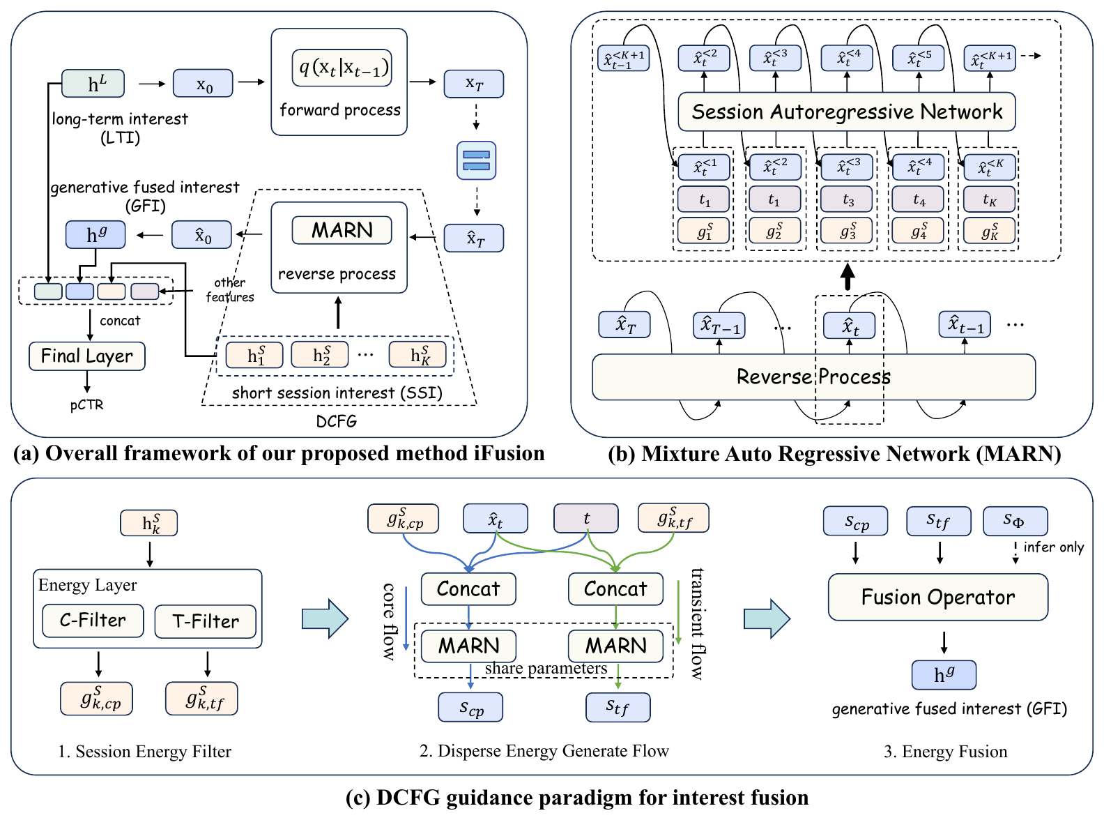
The overall pipeline: fusion as "revising a draft"
The full picture first, then the parts:
| Step | What it does | Output |
|---|---|---|
| Encode | Encode the long-term sequence and each short-term session separately with Transformers | One long-term interest vector, K session interest vectors |
| Add noise | Treat long-term interest as the start and add Gaussian noise step by step as in diffusion | Noisy long-term interest |
| Split signals | Split each session into a stable path and a fluctuation path | Two sets of guidance signals |
| Denoise | Denoise session by session in order with both guidance signals | Fused interest vector |
| Predict | Concatenate fused interest with other features and pass through the final prediction layer | pCTR |
The key division of labor: long-term interest decides "roughly who this person is", short-term sessions decide "which direction to revise now", and how much to revise is controlled by the weights of the two guidance paths. Diffusion models are familiar; what needs explaining is where the supervision comes from. There is no ready-made "right answer" for the fused interest: the vector the network recovers goes straight into the prediction layer and is learned through the click cross-entropy loss, plus an auxiliary loss that asks it to predict the next session's interest (more on this below). So "how well it recovers" is defined by "how well it predicts clicks". At inference no noise is added: following the paper's inference algorithm, the long-term interest is placed as-is at the highest noise level as the starting point, and one or a few recovery steps give the result. Note that training sees noisy inputs while inference sees clean ones, so the two input distributions are not quite the same. The three components follow.
A stable path and a fluctuation path: why split?
The paper calls this component DCFG (disentangled classifier-free guidance). First, what it modifies: classifier-free guidance (CFG) is a common trick in image generation. During training part of the condition is randomly dropped, so the same network learns both "conditional generation" and "unconditional generation"; at inference it takes the unconditional result plus γ times "conditional minus unconditional", and the larger γ is, the more closely the result follows the condition.
The problem is that CFG has only one γ and treats the whole condition the same way. In image generation a text condition like "draw a cat" is clean; in a user's sessions stable preference and impulse are mixed together. Raise γ and the sale-stocking noise is amplified too; lower it and real new interests cannot keep up.
DCFG splits each session into two signals, each with its own weight:
is the interest the network recovers without looking at sessions; is the stable path: first average the representations of all behaviors in the session, then pass the result through an MLP. Averaging dilutes behaviors that appear only once and keeps what recurs, acting like a low-pass filter; the paper says this path's MLP uses stronger regularization but does not give its exact form. is the fluctuation path: attention assigns weights to the behaviors in the session, followed by an MLP. Attention lets a few behaviors take very large weights, so a sudden search is not flattened as it would be in an average, acting like a high-pass filter. Training adds a loss that pushes the inner product of the two signals toward zero, forcing them to handle different things. On a validation set the paper measured an average cosine similarity below 0.102 between the two guidance directions, showing they are indeed mostly separated.
Work through one dimension by hand (illustrative). Suppose a dimension stands for "interest in sports products". Without sessions the network recovers 0.30, with only the stable path 0.50, with only the fluctuation path 0.40. Using the best setting the paper found, weight 2 for the stable path and 1 for the fluctuation path:
The stable path contributes 0.40 and the fluctuation path 0.10. If the fluctuation path has recently been pulled off course by tissues and formula, its bias only counts once, instead of being amplified together with the stable signal as with a single γ. The paper searched 25 weight combinations and found that a stable-to-fluctuation ratio of about 2 works best.
Revising one session at a time: why in order?
The second component is MARN (mixture autoregressive network). The common approach concatenates or pools the representations of K sessions into one condition vector and feeds it to the denoising network at once; the paper calls this non-autoregressive (NAR). MARN processes sessions in time order instead: session 1 guides an intermediate result, which becomes the starting point for session 2, which guides again, and so on.
Why? As an analogy, long-term interest is a draft and each session is an edit note. Merging four notes into one loses the order of "first bought formula for a friend, then looked at running shoes"; revising note by note lets later sessions correct earlier bias and makes the latest intent more likely to survive. Training also has an auxiliary task: predict the interest of session K+1 from the first K sessions, with a cosine distance loss, forcing the model to learn how interest evolves session by session.
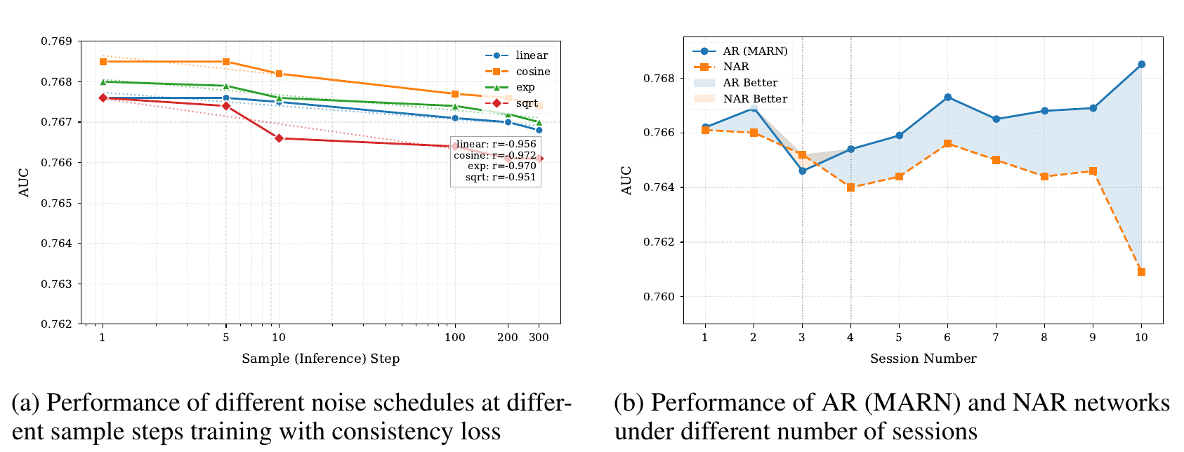
Figure 4(b) is the most direct evidence for this design. With one or two sessions the two approaches are similar; at 10 sessions, processing at once drops AUC to about 0.761 while processing in order stays at 0.7685. This shows that the more sessions there are, the more information lives in their order, and the more a one-shot merge throws away.
What about diffusion being too slow to serve?
The old problem of diffusion models is that inference needs many steps, and a CTR model scores hundreds or thousands of candidates per request, so running 100 steps is unrealistic. The paper adds a consistency loss: pick two noise levels at random and require the network to recover results from the two noisy inputs that are as close as possible. The network thus learns to "go straight to the same answer from any noise level", and the whole reverse process needs only 1 step. Within that step MARN still passes through the K sessions one after another, so what is saved is the number of diffusion iterations; the ordered processing across sessions remains.
Figure 4(a) shows that with the consistency loss, for all four noise schedules more inference steps mean lower AUC; the paper's explanation is that multi-step iteration accumulates error, so the final choice is the cosine schedule (noise strength grows along a cosine curve over the steps, slowly at first and faster near the end) with 1-step inference. In the ablation AUC is almost identical with and without the consistency loss, yet inference is about 25% faster, which shows this loss saves compute without costing quality.
Experiments: how much better is it really?
The experiments use three public datasets and one industrial dataset. Amazon Books takes the most recent 10 behaviors as short-term and the preceding 90 as long-term. Taobao deliberately puts clicks, purchases, add-to-cart and likes into the short-term sequence to test the "feature spaces don't line up" problem; Ali Ads is Alibaba's display ad data. The industrial data trains on about 10 billion click logs from 32 days of a large ad platform and tests on 500,000 from the next day. Baselines cover three groups: classic sequence models such as DIN and DIEN; long-sequence retrieval models such as SIM, ETA and the TWIN family; MTGR; and three diffusion-based recommenders, DiffuRec, DreamRec and DiffuMIN.
| Method | Amazon AUC | Taobao AUC | Ali Ads AUC | Industrial AUC |
|---|---|---|---|---|
| DIN | 0.8162 | 0.8995 | 0.6422 | 0.7564 |
| TWIN-V2 | 0.8433 | 0.9289 | 0.6607 | 0.7634 |
| MTGR | 0.8440 | 0.9296 | 0.6615 | 0.7648 |
| DiffuMIN | 0.8427 | 0.9288 | 0.6595 | 0.7623 |
| iFusion | 0.8512 | 0.9347 | 0.6652 | 0.7685 |
iFusion is first on all four datasets, 0.0037 to 0.0072 above MTGR. More telling are the other three diffusion methods: they trail MTGR on all four datasets and some trail TWIN-V2. This shows that "using a diffusion model" brings no gain by itself; the gain comes from how iFusion uses conditions to guide it.
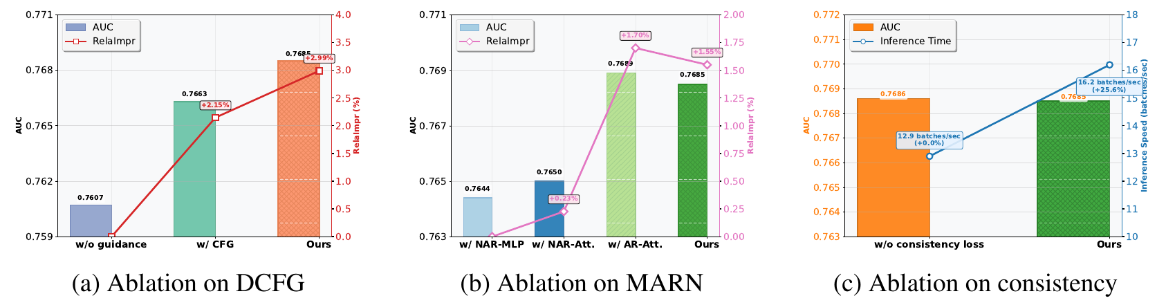
The ablation makes this clearer. With diffusion only and no guidance, industrial AUC is only 0.7607, below MTGR's 0.7648. Standard CFG brings it to 0.7663 and the two-path guidance to 0.7685. In other words, the entire gain over MTGR comes from the guidance scheme, and the step from standard CFG to DCFG contributes 0.0022. Processing sessions in order is about 0.0035 above processing at once, while replacing MARN's internals with a larger attention network adds almost nothing, which shows that what helps is the "in order" structure, not network capacity.
The paper also runs two robustness checks. Plugging the fusion module into three prediction layers, DeepFM, DCN and AutoInt, gives about 0.004 over MTGR in each case; replacing the long- and short-term encoders with the simplest average pooling, iFusion still adds 0.0037. This shows the fusion module can be lifted out and attached to existing models.
Serving cost is low: online TP99 (99th percentile) latency rises only 0.3%, and training time and memory barely change, because inference runs a single step and the only addition is the forward pass of a small network. The 7-day online A/B covered hundreds of millions of users, with CTR up 2.44% and eCPM up 2.61%, showing that the offline gain holds up on real traffic.
Limitations as I see them
First, in its final form "diffusion" is down to one step. Inference runs 1 step, more steps make it worse, and without guidance the diffusion backbone by itself is 0.0041 below MTGR. A more accurate reading is that it learns a session-conditioned function mapping noisy long-term interest directly to fused interest, with diffusion-style training acting more like a regularizer. Separating out what diffusion itself contributes needs one more control: a deterministic network without diffusion that keeps the two-path guidance and in-order session processing. The current ablations do not include it.
Second, the offline gain is not large relative to noise, and the reporting has flaws. The industrial test set is a single day of 500,000 samples, the standard deviation across three runs is about 0.001, and the gain over MTGR is only a little over three times that, so whether the conclusion holds on another day is uncertain. In the appendix's multi-epoch table MTGR's epoch-3 AUC is higher than its epoch-1 AUC, contradicting the text's claim that "all models are best at epoch 1"; it is probably a typo, but it raises questions about how carefully the numbers were checked.
Third, the gap between online and offline is not explained. Offline AUC gains only 0.0037 while online CTR gains 2.44%, a gap that makes sense if the online control is weaker than a strong baseline like MTGR; and with no online ablation, it is unclear which component drives most of the 2.44%. The theory section uses analogies from thermodynamics and energy functions, but the actual implementation is "an average-pooling path, an attention path, plus an orthogonality loss"; readers need not be intimidated by the theorems, nor treat them as evidence for the results.
How a ranking team could try it
- First confirm that long/short-term fusion really is a weak spot: replace the current model's fusion with plain concatenation and see how much AUC drops. If it barely drops, fusion is not the bottleneck and this paper's gain will be limited.
- Start with the cheapest component: skip diffusion, split short-term sessions into an average-pooling path and an attention path, give each a tunable weight, add the orthogonality loss, and see whether it beats a single fusion. This step roughly corresponds to the 0.0022 from CFG to DCFG in the paper.
- If that works, try in-order session fusion. Products with many sessions (for example an e-commerce app users open several times a day) will gain more; products with few sessions can skip it.
- Only then add diffusion training and the consistency loss, fix inference at 1 step, and compare with the deterministic version from steps 2 and 3. If the difference is small, keep the deterministic version, which is simpler to serve and maintain.
One-line conclusion
The key to fusing long- and short-term interest is not switching to a more complex generative model, but weighting the stable part and the momentary fluctuation of short-term signals separately and writing them into long-term interest session by session, in order.
| Dimension | Assessment |
|---|---|
| Problem importance | High. Almost every ranking model with long and short sequences has to fuse them, and most current methods are crude |
| Method novelty | Medium-high. Two-path guidance and in-order session denoising are a new combination; whether diffusion itself is necessary has not been tested on its own |
| Experimental evidence | Medium. Four datasets plus an A/B test over hundreds of millions of users, but the offline gain is only about 3 standard deviations and there is no online ablation |
| Engineering cost | Low. One-step inference, about 0.3% more latency, and it plugs into existing prediction layers |
| Worth trying? | Worth trying the two-path guidance and in-order session fusion; the diffusion part can be validated last |
How did this read for you?
Hoot made a note. Thanks for the feedback.

One tap, no sign-in; tap again to undo. Only anonymous counts are kept, never who you are.
Discussion
Add experiment details, reproduction notes or a different take. Requires a GitHub sign-in.
Loading the discussion…