Contents · 8 sections
1What problem is it actually solving?2Overview: the teacher is a group of agents, the student is one model3How collaborative signals become text4How a group of agents is taught to one model5What the experiments show6Limitations as I see them7How a recommendation team could try it8Conclusion and assessmentSHARE

Teams doing LLM-based recommendation who already have a multi-agent recommendation pipeline that is too slow for production should read this paper, but read it with some skepticism. The paper, from Tencent, tackles a very practical tension: a multi-agent system can reason step by step and call tools, and it works well, but one recommendation takes several hundred seconds on 16 GPUs. The core idea in one sentence: first build a multi-agent teacher that plans, calls collaborative filtering tools and checks its own work, turn the reasoning it got right into one long text, then teach that text to a single 8B model with SFT plus GRPO. The paper calls the teacher MARS (Multi-Agent Recommender System) and the student STAR (Single-agent Trajectory-Aligned Recommender). Across the 5 Goodreads subtasks, the student's average hit rate is 78.4 and the teacher's is 66.2; one inference goes from 461 seconds on 16 GPUs to 89 seconds on 1 GPU (Figure 4). I think the most valuable parts are the tool design, which writes collaborative filtering results as text evidence before handing them to the LLM, and the ablation finding that removing self-checking hurts the most. Keep in mind that "the student beats the teacher" mixes in the gain from in-domain fine-tuning, that the traditional baselines are actually far ahead of STAR on Yelp's interest-drift tasks, and that 89 seconds is still far from production.
What problem is it actually solving?
There are two common ways to use LLMs for recommendation. One treats the LLM as a feature extractor: it produces semantic embeddings that are fused with a collaborative filtering model. Collaborative signals get in, but the LLM's step-by-step reasoning goes unused and the results cannot be explained. The other is agents: the LLM calls tools to look up data and reasons over several rounds. The paper sees two problems with existing agents. First, tools return either scores with no visible reason or raw item attributes, with no group-behaviour information such as "many people bought these together". Second, every extra round of reasoning is one more model call, so latency grows linearly with reasoning depth.
One real sample from the paper's appendix runs through this piece: a Goodreads user who read a large number of children's picture books between 2012 and 2016, with the most recent dozen or so concentrated on the Little Critter series and holiday themes. The system has to pick, out of 20 candidate books, the one this user reads next; 1 of them is the book the user really read, and the other 19 are random. The task is hard in two ways: from titles and blurbs alone, the LLM does not know "people who read this also like what"; and the user's history is too long to fit into the context directly.
Overview: the teacher is a group of agents, the student is one model
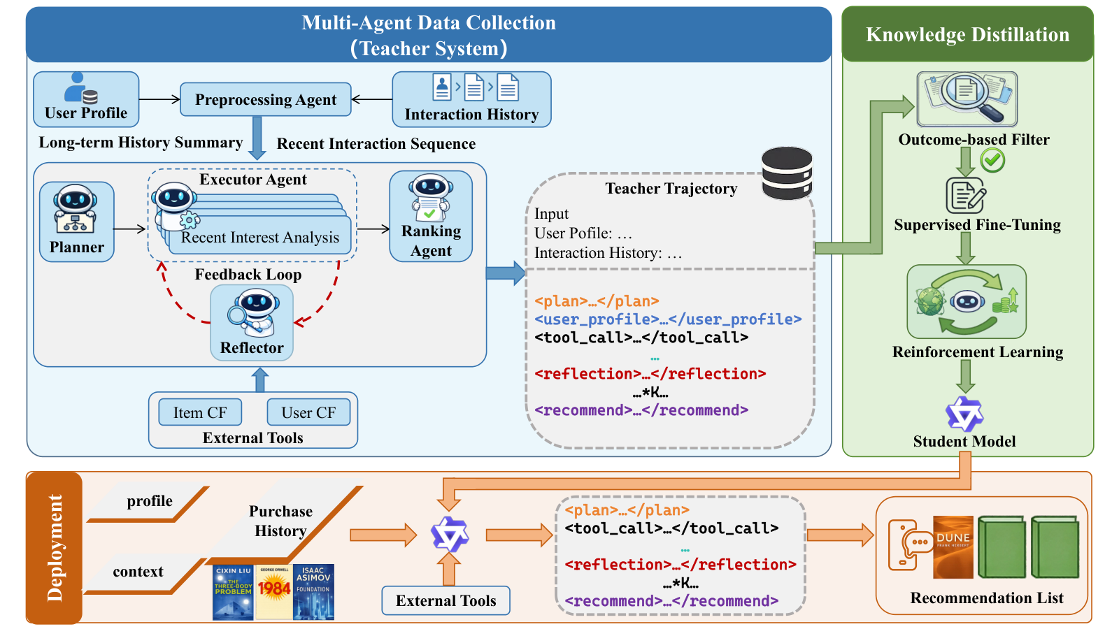
The whole pipeline can be read from this table:
| Stage | What it does | Output |
|---|---|---|
| Preprocessing | Group the user history by time, have an LLM write a rolling summary group by group, keep the last group raw | A long-term summary plus the most recent raw behaviour |
| Teacher reasoning | Plan, execute (4 analysis agents, tools allowed), reflect, redo if needed, rank | A ranking of the 20 candidate books |
| Trajectory serialization | Concatenate the agents' exchanges in order into one tagged text; keep only samples where the teacher's top 1 is right | SFT training data |
| Student training | SFT imitation first, then GRPO with rewards by hit rank | STAR (Qwen3-8B) |
| Deployment | The student generates all stages in one pass; after it writes a tool call, an external system looks up the precomputed text and feeds it back, and the student continues | A ranking |
Concretely, preprocessing works like this: after the history is sorted by time, every m behaviours form a group; the LLM first summarizes the first group, then gets that summary together with the second group and writes a new summary, and so on group by group up to the second-to-last group. The last group stays out of the summary and is concatenated, raw, with the final summary as the teacher's input. In Appendix F.3 the student's input has the same format, a long-term summary plus the most recent raw behaviour, so at deployment this summary also has to be computed in advance. In the appendix sample, behaviour from June 2012 to February 2015 is compressed into one summary, and behaviour after that, up to March 2016, is kept as raw text.
Inside the teacher-reasoning step, things go like this. The planner agent picks the analysis tasks it needs out of 4 and sets their execution order: user profile (extract features and preferences from basic information, behaviour and reviews), long-term interest (summarize stable interests after filtering out anomalous and low-value behaviour), recent interest (look at the immediacy and novelty of recent behaviour), and interest divergence (look for latent interests along three directions: association, scenario, and group commonality). The executor agents complete them one by one in that order, and any of them can call the collaborative filtering tools. The reflector agent reads all the execution results, checks them for consistency, rationality and completeness, points out the problematic sub-tasks and gives revision suggestions; those sub-tasks are re-executed following the suggestions. In the appendix's trajectory template, the re-executed results form their own segment, "Re-executed Sub-task", placed after the reflection. Finally the ranking agent aggregates all the preceding evidence and ranks the 20 candidate books.
The key division of labour is: the teacher's job is to get the reasoning right and write it down; the student only learns that one written trajectory, so in production there are no longer several agents passing messages back and forth. The parts are taken apart below.
How collaborative signals become text
Why is this step needed? An LLM only sees text. Information such as "people who read The Three-Body Problem also often read Dune and Foundation" lives in user-item interaction records, not in any book's blurb. The paper first builds a user-item bipartite graph from all interactions, with users and books as nodes and an edge whenever a user read a book, and then walks the graph in two ways.
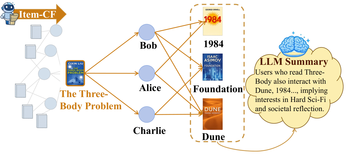
The Item-CF tool walks "book → readers → books": start from a book, find who read it, and collect the other books those people often read. The User-CF tool walks "user → books → users": start from the books the target user read, find other users who also read them, and gather the books those users like. At this point both tools have only a list of books. What differs from other approaches is the next step: an LLM groups the list into a few categories and writes one sentence on what each has in common. In Appendix F.2, starting from the touch-and-feel board book That's Not My Dinosaur, Item-CF returns 5 categories such as "animal-themed picture books" and "interactive and activity-focused books", each with a few representative books.
This step is expensive, since every user and every book needs one LLM call. The paper does all of it offline: the graph and the neighbours are fixed before serving, the summaries are computed once and stored as static data, and a tool call in production is just a lookup. So when STAR "calls a tool" in production, it is a read: the student writes <tool_call>, an external system looks up the table by the arguments, puts the result back into the context as <tool_response>, and the student continues writing. In the Appendix F.3 sample, every tool response is marked with its own arrow, showing it is content fed in from outside, not something the student wrote itself. In the deployment diagram in the bottom half of Figure 1, the external tools are also a separate module. The cost lands on storage; the authors note in their limitations that at billions of users and items, storing a summary for every one of them gets heavy.
How a group of agents is taught to one model
Step one is to turn the teacher's process into one text. Inside the teacher, several agents pass messages to each other; the paper rearranges this into one long text ordered by stage: the plan goes in <plan>, the user profile in <user_profile>, the tool-calling segment keeps <tool_call> and the tool response, then come <reflection> and finally <recommend>. Keeping the tool-call tags matters: the student learns not only the answer but also "when to look up collaborative signals and how". In the Appendix F.3 trajectory for the picture-book user, the reflection stage judges the "interest divergence" step too speculative, pointing out that it suggests graphic novels and fantasy, which conflicts with the user's preference for educational picture books; that step is redone before ranking.
Step two is filtering. Only samples where the teacher's top-ranked book is exactly the user's real next book are kept. Per Appendix Table 3, about 8.6k, 8.0k and 4.7k samples remain for the three datasets. Filtering makes the student imitate only reasoning that got the answer right, not the routes the teacher took when it guessed wrong.
Step three is SFT. Full-parameter fine-tuning on these trajectories teaches the student to write stage by stage and call tools in the right format.
Step four is GRPO. SFT only copies; the authors then use reinforcement learning so that the student finds better ways of writing among its own outputs. For each question, 8 outputs are sampled, and each output's reward is a format score plus a rank score:
is the -th output and is the user's real next book. The format score is +1 when all required stage tags are present and the tool-call syntax is valid, and −1 otherwise. The rank score is 1 if the real book is ranked first, 2/3 if it is in the top 3, 1/3 if it is in the top 5, and 0 otherwise.
A hand-computed illustration: among 8 outputs for the same question, A has a valid format and ranks the real book second, scoring ; B ranks the real book first but drops the reflection tag, scoring ; C has a valid format but the real book is not in the top 5, scoring 1. GRPO compares the 8 rewards with each other: A is above the group average, so its way of writing is reinforced; B, although correct, is pushed down for breaking the format. The intuition behind this design is that the format score preserves the habit of reasoning in stages and calling tools with valid syntax, while the rank score pushes the student to move the real book up.
The GRPO training questions are chosen on purpose: the SFT model samples each question 8 times, and questions are split by the number of successes into easy (6–7), medium (3–5) and hard (1–2), mixed 3:4:3, giving only about 500 questions per dataset. The appendix only uses the phrase "success count", so the criterion for whether one output counts as a success is left to whoever reproduces it, for example the real book ranked first, or the real book in the top 5 with a valid format; the two criteria produce different bins. Questions with 0 or 8 successes fall into none of the three bins, so the training set uses only the questions in between, where the student is sometimes right and sometimes wrong. This shows the reinforcement learning budget is spent entirely on questions the student has not yet mastered reliably. One more gap: the paper does not say whether sampling in the GRPO policy optimization stage, when it hits a tool call, runs the real retrieval and feeds the result back, or lets the model generate the tool response itself. When reproducing, keep it consistent with deployment: pause generation during sampling too and feed back the real tool result, otherwise the student may learn to make up tool responses.
What the experiments show
Evaluation follows the protocol of AgentRecBench (a public benchmark for agent recommender systems) on three datasets: Amazon, Goodreads and Yelp. Each dataset has 5 subtasks: classic recommendation, user cold start, item cold start, long-term interest and short-term interest, with 100 samples per subtask and 1,500 in total. Each sample has only 1 correct book among 20 candidates, and the metric is the average of HR@1, HR@3 and HR@5. All agent baselines use DeepSeek-V3, and so does the teacher MARS.
First, a reference point: ranking 20 candidates at random gives HR@1 of 5%, HR@3 of 15% and HR@5 of 25%, which average to exactly 15.0. In Table 1, MF and LightGCN score 15.0 on every classic and cold-start task, the same as random. This shows that under this protocol the traditional models learn essentially nothing on these tasks, so using them as baselines says little.
| Method | Amazon classic | Goodreads user cold start | Yelp classic | Yelp long-term interest | Yelp short-term interest |
|---|---|---|---|---|---|
| LightGCN | 15.0 | 15.0 | 15.0 | 31.6 | 68.9 |
| RecHacker | 63.0 | 49.3 | 7.0 | 9.3 | 7.7 |
| MARS (teacher) | 68.4 | 63.7 | 31.0 | 20.3 | 13.3 |
| STAR (student) | 79.0 | 76.3 | 43.0 | 23.0 | 17.7 |
STAR leads across Amazon and Goodreads; on the Amazon classic task it scores 79.0, against 63.0 for RecHacker, the runner-up of the challenge.
Yelp is a different picture. Every agent method is low there, and STAR scores only 12.3 and 11.3 on the two cold-start tasks, below the random 15.0. On the interest-drift tasks it is the other way round, with the traditional models strong: LightGCN scores 68.9 on short-term interest, STAR 17.7. This shows that the main text's claim that "STAR outperforms both traditional and agent baselines on all datasets" does not match these cells of its own Table 1. The abstract's "the student beats the teacher by 8.7% to 39.5%" is a relative gain, and the largest, 39.5%, comes from Yelp item cold start, from 8.1 to 11.3; because the base is so small, the relative number looks large.
All ablations are on Goodreads, and the numbers are averages over the 5 subtasks:
| Variant | Teacher MARS | Student STAR |
|---|---|---|
| Full | 66.2 | 78.4 |
| Without tools | 61.6 | 72.8 |
| Without planner | 65.3 | 76.9 |
| Without reflector | 62.4 | 71.9 |
| Without GRPO | — | 75.5 |
In the student column, removing reflection costs 6.5 points, the most of any component, and more than the 3.8 points the teacher loses without reflection. The authors' explanation is that the filtered data still consists of correct samples, but without the "find the error, go back and redo" segment, the student never learns to recover from errors made midway. Removing tools costs 5.6 points, which shows the collaborative-signal text written offline really helps. GRPO adds 2.9 points (75.5 to 78.4). This shows that on this task, teaching the model to check and correct its own reasoning matters more than teaching it to split the task.
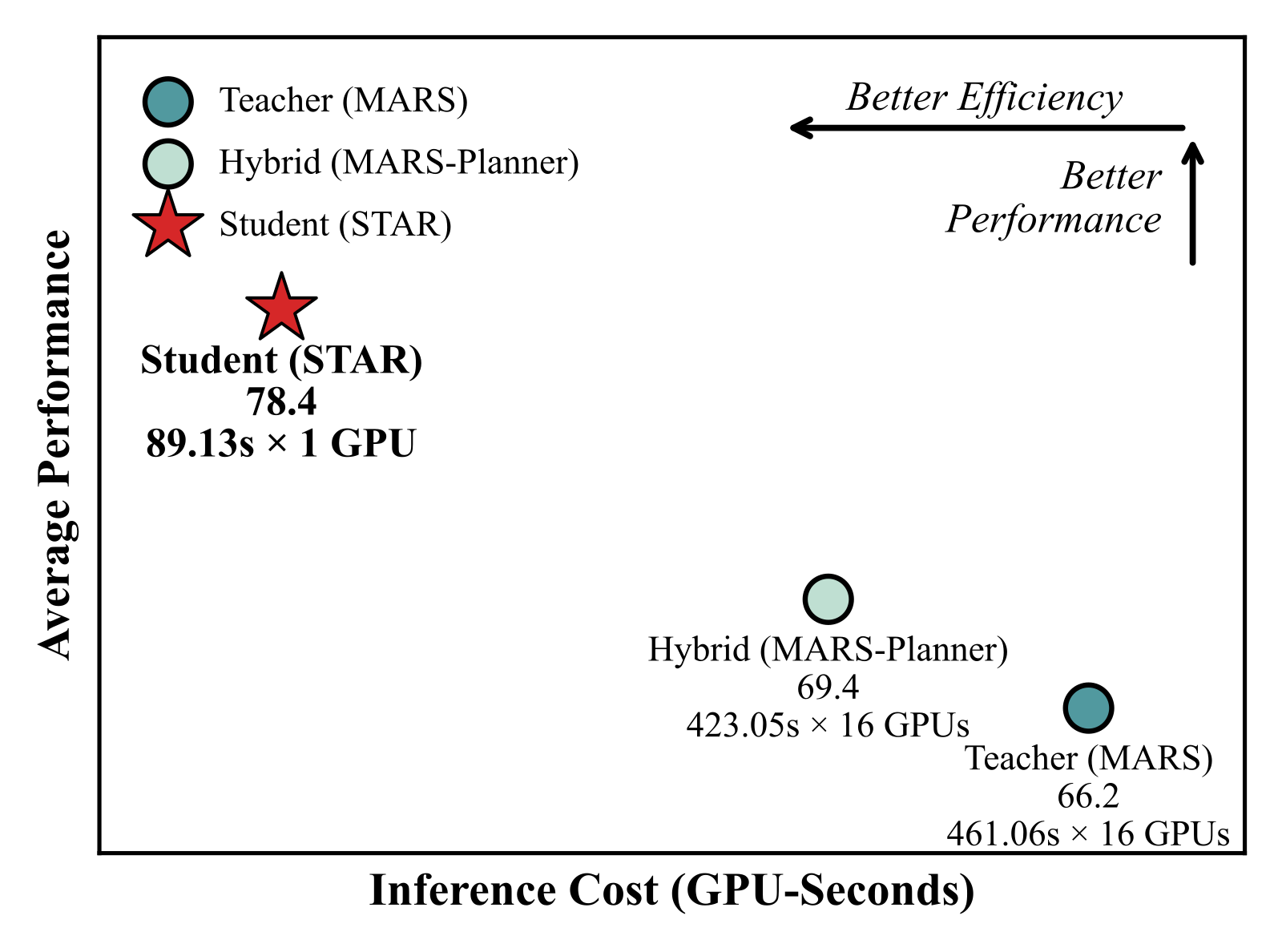
Figure 4 also has a control: replacing only the planner agent with a fine-tuned Qwen3-8B, while every other agent still uses DeepSeek-V3, scores 69.4 and lowers the cost only from 461 to 423 seconds. This shows that distilling a single stage saves little; the cost only drops once the whole pipeline is merged into one model. In GPU-seconds, 461 seconds on 16 GPUs versus 89 seconds on 1 GPU is a gap of about 80x.
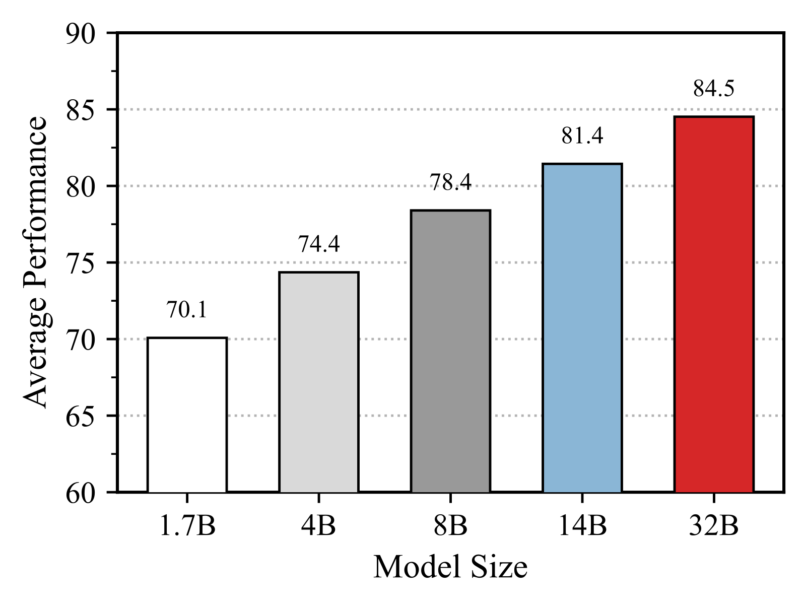
Going from a 1.7B to a 32B student raises the Goodreads average from 70.1 to 84.5. Even the 1.7B student is above the teacher's 66.2.
Limitations as I see them
First, "the student beats the teacher" cannot all be credited to the distillation method. The teacher is DeepSeek-V3 with no fine-tuning at all, while the student gets full-parameter fine-tuning on about 8k samples from the same benchmark and the same kinds of tasks, then reinforcement learning on about 500 questions. That even the 1.7B student beats the teacher shows in-domain training is strong on its own. The paper lacks a control: fine-tune directly on the same samples with only "history + candidates + correct answer", without the reasoning trajectory, and see how far that gets. Without that row, there is no way to tell whether the gain comes from the reasoning trajectories or from in-domain supervision.
Second, the evaluation is small and narrow. Each subtask has 100 samples, so one sample in a subtask is worth 1 point of HR@1, and removing the planner differs by only 1.5 points, which is hard to separate from noise. There are only 20 candidates with randomly drawn negatives, and the authors admit it is unknown what happens with full-corpus ranking.
Third, it is still far from deployment. At 89 seconds per recommendation, it is more than two orders of magnitude away from the sub-second latency production needs; the offline summaries have to cover every user and every book, and the authors themselves say storage is a problem on billion-scale platforms. There is also a textual inconsistency: the main text says SFT used 3 epochs, a learning rate of 2e-5 and batch size 16, while Appendix Table 4 says 2 epochs, 1e-5 and a global batch size of 64; watch for this when reproducing.
How a recommendation team could try it
- Start with only the tool layer. Run Item-CF offline for popular items, hand the neighbouring books to an LLM to group and describe in a few sentences, and feed that as extra input to an existing LLM ranker or to recommendation-reason generation. Measure offline metrics and human ratings of the reasons; this step needs no agents at all.
- Then run a control experiment to see whether the reasoning trajectory is worth it. Train two students on the same data: one learns only the final ranking, the other the full trajectory. If the gap is small, there is no need to build a teacher.
- If trajectories help, keep the reflection-and-redo segment first, since it contributes the most in the ablation. Keep only training samples the teacher got right.
- Only then consider the serving form. An 89-second inference fits only latency-tolerant settings such as offline re-ranking or daily-refreshed recommendation reasons; to get into the real-time path, you would at least need a smaller model and shorter trajectories.
Conclusion and assessment
The key takeaway: collaborative filtering results can first be written as a paragraph of text evidence and then handed to an LLM to reason over; and the part of a multi-agent system that is really worth distilling is the segment where it checks and corrects its errors.
| Dimension | Assessment |
|---|---|
| Problem importance | Medium-high. The tension between quality and latency is the core obstacle to deploying LLM recommendation |
| Method novelty | Medium. Distilling multi-agent systems into one model has precedents; what is new is the tool that writes collaborative filtering results as text, and a trajectory format that keeps tool calls and reflection |
| Experimental evidence | Medium to weak. The ablations are complete, but each cell has only 100 samples and there are only 20 candidates; it lacks a fine-tuning control without trajectories; it trails traditional models on Yelp |
| Engineering cost | High. You need a multi-agent teacher and offline summaries for every user and item, and one student inference still takes 89 seconds |
| Worth trying? | Try the tool layer first: writing collaborative neighbours as text offline is the cheapest piece and the easiest to validate on its own |
How did this read for you?
Hoot made a note. Thanks for the feedback.

One tap, no sign-in; tap again to undo. Only anonymous counts are kept, never who you are.
Discussion
Add experiment details, reproduction notes or a different take. Requires a GitHub sign-in.
Loading the discussion…