SHARE

Teams building generative recommenders should read this. It does not change the model architecture; it answers a practical question: if you already have a well-trained classic sequential recommender, how do you teach what it knows to a new model that recommends through Semantic IDs? The core idea in one sentence: the old model outputs probabilities over "which item comes next", the new model predicts "what each code position is", and the paper gives two conversion routes that move the former into a form the latter can learn directly. The effect is concrete: on Amazon Beauty, Recall@10 rises from 0.0940 to 0.1094; averaged over three datasets, the first route lifts Recall@10 by 15.39% and the second lifts NDCG@10 by 8.28%.
What problem is it actually solving?
Semantic-ID recommendation gives every item a short string of discrete codes, such as the three-position code (0, 1, 2), and recommends by predicting the next item's code. The codes are quantized from each item's semantic representation (here 16 subspaces with 3 residual levels each, giving 48 positions of 256 values), fixed before distillation and unchanged during training. This paper studies the "parallel" family: the model predicts all code positions at once instead of generating them one by one like TIGER. To rank items, it averages the log-probabilities of each item's codes.
These models are normally trained with hard labels: whichever item the user picked next, every position must predict that item's code, and everything else counts as wrong. That tells the model the right answer but says nothing about how close the other candidates were.
An illustrative example: a user recently bought baby body wash and a bath toy, and the next purchase was a towel. The hard label says "towel right, everything else wrong". A trained SASRec would say: towel 50%, baby bathtub 30%, bib 15%, power bank 5%. The bathtub is as sensible as the towel; the power bank is unrelated. Hard labels carry none of this nuance.
| Candidate (illustrative) | Code | Hard label | SASRec probability |
|---|---|---|---|
| Towel (actual next item) | (0, 1, 2) | 1 | 0.50 |
| Baby bathtub | (0, 2, 1) | 0 | 0.30 |
| Bib | (1, 1, 2) | 0 | 0.15 |
| Power bank | (2, 0, 0) | 0 | 0.05 |
The difficulty is that the two models speak different languages: SASRec gives probabilities over ten-thousand-plus items, while the new model outputs probabilities per code position. Knowledge distillation here means converting the former into targets the latter can learn.
The pipeline: one teacher, two conversion routes
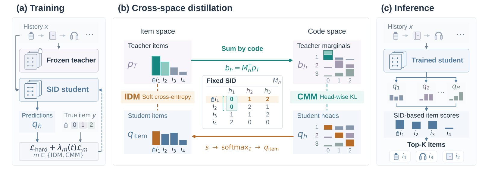
The pipeline has three steps:
- Train an ordinary SASRec as the teacher and freeze it. For each user history it gives probabilities over all items.
- The student is a parallel code model that learns hard labels as usual plus one distillation objective, either IDM (item distribution matching) or CMM (code marginal matching), trained separately.
- At serving time only the student runs, exactly as before, with no extra cost.
One way to remember the split: IDM moves the student toward the teacher and aligns at the item level; CMM moves the teacher toward the student and aligns per code position.
Route one: rebuild items from the student, then compare (IDM)
Why is this needed? The teacher talks about items and the student talks about codes, so the most direct fix is to translate the student into items. Each item's score is the average of its per-position code scores; a softmax over all items gives the student's probability of "which item is next", and a cross-entropy pulls it toward the teacher's distribution.
This has a side effect. Many items share a code at some position; the towel and the bathtub both have 0 in position one. Raising the score of code 0 in position one lifts both. Because the softmax runs over the whole catalogue, lifting one group pushes others down, so all positions are trained together through this step. IDM optimizes exactly the score used for ranking, so it is better at pulling the right items into the top results.
Route two: spread the teacher's probabilities onto each code position (CMM)
The other route translates the teacher into codes. For each position, add up the probabilities of items that share a code there, giving a target probability for each code value:
Here is the user history, is the teacher's probability for item , is item 's code at position , and is the target probability that position takes code . Intuitively it answers: "according to the teacher, how likely is the next item's position to be ?"
With the table above (illustrative): towel and bathtub both have 0 in position one, so code 0 gets 0.50 + 0.30 = 0.80; only the bib has 1, giving 0.15; only the power bank has 2, giving 0.05. Position two differs: towel and bib share code 1, totalling 0.65, and the bathtub's code 2 gets 0.30. The hard label would only say "code 0 at 100%" for position one.
Each position then uses a KL divergence to pull the student's prediction toward its target. Why is per-position matching enough? The yardstick is the KL divergence between the teacher's distribution over complete codes and the student's distribution formed by multiplying its per-position predictions. The authors prove that the student-dependent part of that divergence equals the sum of the per-position KL terms, so with independent positions the optimum is to make each position match its target. CMM calibrates each position directly, so it is better at ordering the top results correctly.
Why tune the distillation weight separately?
The student's objective is "hard-label loss + weight × distillation loss". The two losses naturally have different gradient sizes: a hard label concentrates all error on one answer, while a soft target spreads it over many candidates. The authors run a few early batches, compute each loss's gradient over all trainable parameters, take the L2 norms, and form the ratio "hard-label norm ÷ distillation norm". The median ratio becomes a scaling factor, multiplied by a chosen strength. This makes "strength 1" mean roughly the same thing across datasets and objectives. The distillation weight also ramps up from small at the start of training.
Do the two routes actually help?
The student follows AsymRec's structure, with 48 code positions and 256 values per position. Data are the Beauty, Toys, and Sports categories of Amazon 2014, with 12k to 18k items each. The control is the same architecture trained only with hard labels, which is also the strongest baseline. The table shows Recall@10 and NDCG@10 from Table 2 of the paper, averaged over three runs:
| Method | Beauty R@10 | Beauty N@10 | Toys R@10 | Toys N@10 | Sports R@10 | Sports N@10 |
|---|---|---|---|---|---|---|
| TIGER | 0.0648 | 0.0384 | 0.0712 | 0.0432 | 0.0400 | 0.0225 |
| RPG | 0.0798 | 0.0454 | 0.0885 | 0.0485 | 0.0435 | 0.0249 |
| AsymRec (hard labels) | 0.0940 | 0.0547 | 0.1002 | 0.0586 | 0.0573 | 0.0322 |
| IDM | 0.1094 | 0.0590 | 0.1176 | 0.0638 | 0.0644 | 0.0333 |
| CMM | 0.1069 | 0.0592 | 0.1144 | 0.0647 | 0.0639 | 0.0341 |
Both routes beat hard-label training on all three datasets; on Toys, Recall@10 rises from 0.1002 to 0.1176. This shows that with the architecture, codes, and inference unchanged, adding the teacher's nuance to the training target clearly improves retrieval. The split is stable too: IDM has higher Recall and CMM higher NDCG everywhere, matching the mechanisms.
The ablation asks which part of the teacher's information matters. Keeping only the teacher's top item, or spreading the remaining mass uniformly, both do worse than the full distribution; on Beauty, IDM's Recall@10 drops from 0.1094 to 0.1041 with only the top item. So what helps is the teacher's graded scores across candidates, not just one more answer.
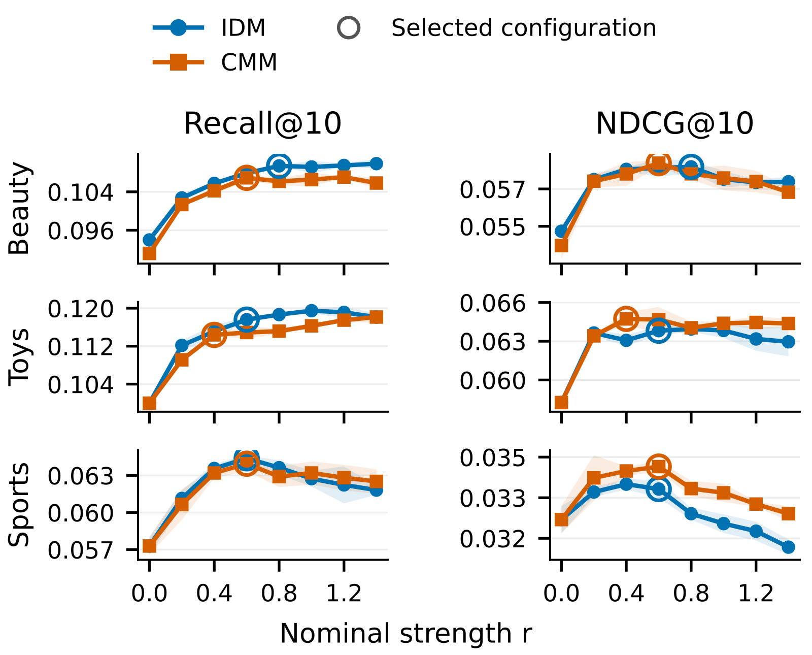
The strength sweep (Figure 2 below) shows that any positive weight beats no distillation on Recall@10, but NDCG@10 falls back when the weight is too large. The teacher mainly helps find more plausible candidates; the exact order at the top still relies on hard labels. Averaging the scores of two separately trained students reaches NDCG@10 of 0.0597 on Beauty, higher than either alone, while training both objectives in one student does not.
Limitations as I see them
First, results depend heavily on the teacher. With a teacher trained on 25% of the data, IDM's Recall@10 on Beauty is 0.0934, below the hard-label 0.0940. A weak teacher hurts.
Second, sensitivity to how peaked the teacher's probabilities are. Flattening them with temperature 4 (the default is 1) drops CMM's Beauty Recall@10 to 0.0881, also below its hard-label baseline. Temperature and weight must be tuned on validation data.
Third, the experiments are small. Each dataset has only 12k to 18k items, and IDM needs a softmax over the whole catalogue per sample; the cost at tens of millions of items is not discussed.
How a recommendation team could try it
- The teacher need not beat the code model. In the paper, the SASRec teacher's own Recall@10 is clearly below the hard-label parallel student on all three datasets, yet distillation still helps, so try an existing sequential model rather than ruling it out for being weaker.
- Try CMM first. It sums teacher probabilities by code into a per-position target; building that target touches every item, but the student only matches a distribution over the code vocabulary at each position, and it plugs into existing training easily. Watch NDCG@10.
- Then try IDM for recall. With a large catalogue, run the softmax over a candidate subset first.
- If both help, try equal-weight score fusion, which needs no retraining.
Verdict
The key lesson: hard labels only say which item is right; the teacher's probabilities also say how wrong the others are, and a code model can learn that by simple summing or averaging.
| Dimension | Assessment |
|---|---|
| Problem importance | High. Code-based models are spreading, and reusing existing sequential models is a common need |
| Novelty | Medium. Distillation is not new; the contribution is two conversion routes and a clear account of their strengths |
| Evidence | Medium. Three datasets, three runs, significance tests, but small data and no online test |
| Engineering cost | Low to medium. CMM adds almost nothing; IDM must handle a full-catalogue softmax on large catalogues |
| Worth trying | Yes. Teams with a sequential model moving to code-based models can validate cheaply with CMM first |
How did this read for you?
Hoot made a note. Thanks for the feedback.

One tap, no sign-in; tap again to undo. Only anonymous counts are kept, never who you are.
Discussion
Add experiment details, reproduction notes or a different take. Requires a GitHub sign-in.
Loading the discussion…