 CIKM 2026
Contents · 11 sections
1What problem does it actually solve?2The URM pipeline3Why 128 readout slots?4How do you learn a table of tens of millions of items?5How do you score only a small part of tens of millions of items?6Experiments: how many dedicated channels can one model replace?7What changes when you change the objective sentence?8Online: run asynchronously, store, then use9Limitations as I see them10How a recommendation team could try it11VerdictSHARE

Teams that run recommendation retrieval and maintain several dedicated retrieval models should read this. In this CIKM paper from Alibaba's Taobao and Tmall Group, one large language model handles click retrieval, per-scenario retrieval, long-tail retrieval, interest exploration and retrieval with a search query at the same time, and overall does better than the multi-task retrieval models common in industry. The core idea in one sentence: the user's history and the goal of this retrieval are written into one input, the LLM outputs several user vectors in a single forward pass, takes inner products with the vectors of tens of millions of candidate items, and keeps the highest-scoring set; switching objectives only means switching that objective sentence. The paper calls it URM (Universal Retrieval Model).
On 9 retrieval objectives in industrial data, URM's average R@1000 is 0.403 against 0.363 for the strongest multi-task baseline, an average relative gain of 11.0%, and it is best on 6 of the 9. To make the LLM affordable over tens of millions of candidates, the authors score only a few tens of thousands of items each time, cutting the compute of the item-scoring step from about 5000 GFLOPs to about 2 GFLOPs. In an online A/B test on an advertising platform, the core metric, advertising revenue, rose 3.01%. What really matters is one model that switches retrieval objectives on instruction: retrieval channels no longer each need their own training, and a new objective close to the learned ones can be tried by changing one sentence. The authors also admit that objectives far from the training objectives still need more training data.
What problem does it actually solve?
Online recommendation usually runs multi-channel retrieval: one channel retrieves by clicks, one by purchases, one looks only for long-tail items, one shows users new categories they have not browsed, and each scenario (home feed, item page and so on) may have its own channel. Each channel has its own training data and model architecture and is trained, evaluated and deployed separately. When an objective changes, a new dataset must be collected and a new channel trained. New objectives also often lack enough samples.
Picture a user (illustrative) who recently favorited a pair of running shoes, bought sports socks and clicked a few quick-dry shirts. Different objectives want different items back:
| Objective (illustrative) | What it should retrieve | Traditional approach |
|---|---|---|
| Click prediction retrieval | The running gear the user is most likely to click next | One two-tower or sequence model |
| Interest exploration | A category the user has never browsed, such as cycling gear | Another model, another dataset |
| Long-tail retrieval | Low-sales but relevant running shoes from small shops | Yet another model |
| Retrieval with a query | Waterproof running shoes when the user searches "waterproof" | A three-tower model with a separate query tower |
URM's answer: all four rows use the same model, and the only difference is the objective sentence at the end of the input, such as "Please retrieve items that the user will click on" or "Please retrieve items from new categories".
The URM pipeline
| Step | What happens | Output |
|---|---|---|
| 1. Build the input | User attributes, statistical features and behavior sequences are written as text, with past items embedded as item IDs; an objective sentence follows, then M readout slots | A sequence of at most 1024 positions |
| 2. LLM forward | Qwen-7B, fully fine-tuned, runs one forward pass | Each of the M readout slots gives one user vector |
| 3. Scoring | Each user vector takes an inner product with item vectors; an item's score is the largest of its M inner products | Item scores |
| 4. Sampling | Instead of scoring all tens of millions of items, only the few tens of thousands picked by a few sampling rounds are scored | The final 1000 items |
Items in the input are not text but special tokens. With billions of item IDs, they cannot fit in the LLM's vocabulary, so the authors keep a separate distributed hashtable that looks up an item vector by ID, and a one-layer MLP maps it to the same size as a text token. This input-side table covers the billion-scale items in behavior sequences and is not the same table as the item table of tens of millions of candidates used for scoring later. When a type of behavior is empty, that sentence is simply dropped, and sequences are truncated but never padded. This costs less compute than fixed-length feature inputs and copes better with missing features.
The key division of labor: the LLM understands this user and this objective, a factorized item table turns that understanding into scores over tens of millions of items, and sampling computes only the small part that could matter. The pieces follow.
Why 128 readout slots?
The most direct form of generative retrieval has the LLM output one user vector at the last position and compare it with every item. The problem is that one vector struggles to represent several interests at once: running shoes and cycling gear may sit far apart in item space, and a single vector can only land in between.
URM appends M fixed placeholder tokens (the paper calls them query tokens), here called readout slots. Each slot has its own learnable embedding, and the LLM outputs one user vector at each slot, so one forward pass yields M of them. Because attention runs only forward, later slots can see what earlier slots produced, so different slots learn different sides of the user's interests. An item's score is the maximum of its inner products with the M user vectors. The authors say they tried weighted sums of these products and the maximum worked better.
A tiny example (illustrative): two slots, one leaning to running and one to cycling. Running shoes score 0.9 and 0.1 against the two user vectors, a cycling helmet 0.2 and 0.8. After taking the maximum they score 0.9 and 0.8, and both reach the top. With one compromise vector both might sit around 0.5 and be pushed out by more "average" items.
The appendix shows the gain is not just from more dimensions. On click prediction retrieval (CPR), 32 readout slots of 128 dimensions each reach R@1000 of 0.248. One slot that outputs 4096 dimensions, then cut into 32 pieces of 128 dimensions, has the same total size yet reaches only 0.163; raising item vectors to 4096 dimensions as well reaches only 0.203. The main text uses 128 slots by default, and more slots give better results.
How do you learn a table of tens of millions of items?
In the last step, "user vector × item table", the table W has one column per item. With tens of millions of candidates it has too many parameters and is hard to learn. Earlier generative retrieval avoids this table by encoding each item as a few levels of short Semantic ID codes, but that requires several LLM calls to generate level by level. A 1.5B model already takes about 50 ms for one pass at length 1024, which is the latency limit of the authors' online retrieval, so URM insists on a single forward pass and shrinks the table instead.
The method is W = U·Vᵀ. U is a small projection that compresses the 4096-dimensional LLM output to 128 dimensions; V holds one 128-dimensional vector per item. Each item vector is the sum of two parts: Hoot says

Item seen in training
- discriminative part V_dis
- one learnable row per item, initialized from two-tower ID embedding
- transferable part V_trans
- item text encoded by a text-embedding LLM, then a learnable linear layer to 128 dims
- item vector
- sum of both parts
Discriminative part alone: 0.256 R@1000 on all items; both parts: 0.263.
Item unseen in training
- discriminative part V_dis
- not used: the paper scores these items with W = U·V_transᵀ
- transferable part V_trans
- the same text path still produces it
- item vector
- transferable part only
Table 3: adding the transferable part lifts R@1000 on unseen items from 0.116 (discriminative only) to 0.130.
The paper's contribution is one LLM that retrieves by objective sentence; this table unpacks the item table W = U·Vᵀ it rewrites so that one forward pass is enough. Numbers are the paper's R@1000 ablation on the CPR objective. Source: paper §3.2 item-table factorization and Table 3
- Discriminative part (V_dis): one row of free learnable parameters per item, initialized from the two-tower model's ID embedding. For items with plenty of training data it separates similar items.
- Transferable part (V_trans): the item's title, category, price, shop, and last-7-day sales and click-through rate are written as text, encoded by a text-embedding LLM, and compressed to 128 dimensions by a learnable linear layer. New items never seen in training have only this part, and it lets them be retrieved.
The ablation shows each part covers one side. On CPR, the discriminative part alone gives R@1000 of 0.256 on all items and 0.116 on unseen items; the transferable part alone gives 0.152 and 0.101; their sum gives 0.263 and 0.130. So the discriminative part carries overall quality, the transferable part adds new items, and together both numbers are best.
Training also avoids a softmax over all items. Positives are compared only with sampled negatives: each batch samples 10,000 negatives in proportion to item frequency raised to the 3/4 power, and each item's score is again the largest inner product over the M readout slots.
How do you score only a small part of tens of millions of items?
At inference, taking inner products with 10 million items for every user is too expensive. The simplest shortcut is to score a random subset, but the items the user actually wants may never be drawn. URM instead expands outward from promising items: it builds a nearest-neighbor index on the item table and then repeats "score, sample by probability, expand to neighbors".
The algorithm starts from a batch of candidate items picked at random, and then each round does three things:
- Compute probabilities for the current batch with the same user vectors (temperature 0.07).
- Sample 1000 items by probability (rather than taking the top 1000, which gives items ranked 1000th and 1001st a fairer chance).
- Add up to 32 nearest neighbors of each of those 1000 items; together they form the batch scored in the next round.
This runs for 4 rounds and returns the 1000 items sampled in the last round.
This relies on one assumption: items close together in the item table score similarly for the same user. Every round reuses the same user vectors, so the LLM is never run again.
Working out the scale: from the second round on, each round scores at most 1000 × (32 + 1) = 33,000 items, against about 10 million in full, which means each round touches about 0.3% of the catalog.
The paper puts the same saving in compute terms. With its settings (128 slots, 4 rounds), projection plus sampled scoring costs about 128 × 128 × (4096 + 4 × 1000 × 32) ≈ 2.2 × 10⁹ operations, which means about 2 GFLOPs. Full scoring costs about 128 × 4096 × 10⁷ ≈ 5.2 × 10¹², about 5000 GFLOPs, so the scoring step becomes small next to the LLM itself.
The sampling-rounds experiment shows 4 rounds are basically enough. The authors measure offline how much sampling recovers as "R@1000 with sampling ÷ R@1000 with full scoring": 1 round gives only 0.2%, 2 rounds 2.1%, 3 rounds 41.7%, 4 rounds 91.0% and 5 rounds 91.1%. My reading is that the start is random, so the first two rounds are still moving toward the user's interest region and recover almost nothing.
Experiments: how many dedicated channels can one model replace?
The industrial dataset comes from online logs, with hundreds of millions of samples and tens of millions of candidate items. Each user's behavior over one day forms the target set; earlier days are used for training and the next day for testing. Baselines are the two-tower, Transformer sequence and Attention-DNN models common in industry, each in a single-objective (single-task) and a multi-objective (multi-task) version; the best of them, Attention-DNN, also gets Shared Bottom, MMoE and PLE multi-task structures. R@1000 excerpt (the scene B and purchase prediction columns are left out; URM is also first on both):
| Model | CPR | Scene A | Scene C | Exploration SR | Long-term LR | Long-tail LIR | Query RQ | Avg of 9 |
|---|---|---|---|---|---|---|---|---|
| Two-tower single-task | 0.129 | 0.271 | 0.129 | 0.069 | 0.066 | 0.117 | 0.355 | 0.161 |
| Attention-DNN single-task | 0.253 | 0.477 | 0.260 | 0.106 | 0.213 | 0.251 | 0.651 | 0.323 |
| Attention-DNN multi-task | 0.238 | 0.456 | 0.277 | 0.062 | 0.336 | 0.265 | 0.671 | 0.351 |
| Attention-DNN Shared Bottom | 0.243 | 0.442 | 0.270 | 0.072 | 0.337 | 0.224 | 0.745 | 0.357 |
| Attention-DNN PLE | 0.256 | 0.451 | 0.274 | 0.062 | 0.327 | 0.224 | 0.761 | 0.363 |
| URM | 0.263 | 0.530 | 0.362 | 0.093 | 0.285 | 0.240 | 0.835 | 0.403 |
The table shows two things. First, traditional multi-task learning has a seesaw: moving Attention-DNN from single-task to multi-task lifts long-term interest from 0.213 to 0.336 but drops exploration from 0.106 to 0.062. Second, URM does not win everywhere: it is first on 6 objectives (click, purchase, the three scenes and query retrieval) and still loses to the best baseline on exploration, long-term interest and long-tail. Query retrieval stands out: a three-tower model with a dedicated query tower reaches 0.822, and URM reaches 0.835 with no special structure, so the two are comparable.
On 4 public datasets (Amazon Sports, Beauty, Toys and Yelp), URM's HR@5 and NDCG@5 are on average 46% and 29% higher than the strongest baseline (including Semantic ID methods such as TIGER). These datasets are small and mainly show the method works; the industrial table says more.
What changes when you change the objective sentence?
This part shows best what "universal retrieval" means: the same model, with only the objective sentence in the input changed.
- Per scenario: for the same users, retrieving with the "scene A" sentence gives scene A an R@1000 of 0.530, against 0.440 with the generic click-retrieval sentence. Relative gains across the three scenes range from 20.5% to 31.0%. The model really reads the sentence and adjusts its output by scenario.
- Interest exploration: switching to "Please retrieve items from new categories" raises the share of new-category items in the results from 18.8% to 46.2% and exploration R@1000 from 0.051 to 0.093. The cost is click retrieval falling from 0.263 to 0.213, so objectives really trade off; the gain is not free.
- A combination never trained: training has only the query objective and the long-tail objective separately; at test time the two sentences are joined. Query retrieval R@1000 is 0.836, level with 0.835 using the query objective alone, while the long-tail share of the results rises from 79.6% to 82.4%. Adding the long-tail request did not cost any match with the search query.
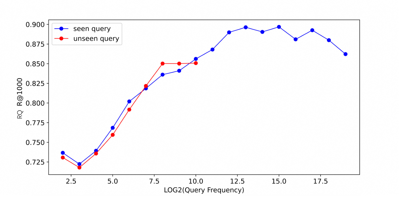
For queries unseen in training, the authors group queries by how common they are (occurrence frequency, log2 on the x-axis) and plot the results (the second figure above). "Seen" means the query appears in the training data, which is a different thing from how common it is: an uncommon query may simply have missed the training data. At the same frequency, seen and unseen queries have almost the same recall. Unseen queries are mostly long-tail terms with a different distribution from common ones, so comparing them at matched frequency is what makes the comparison fair.
Online: run asynchronously, store, then use
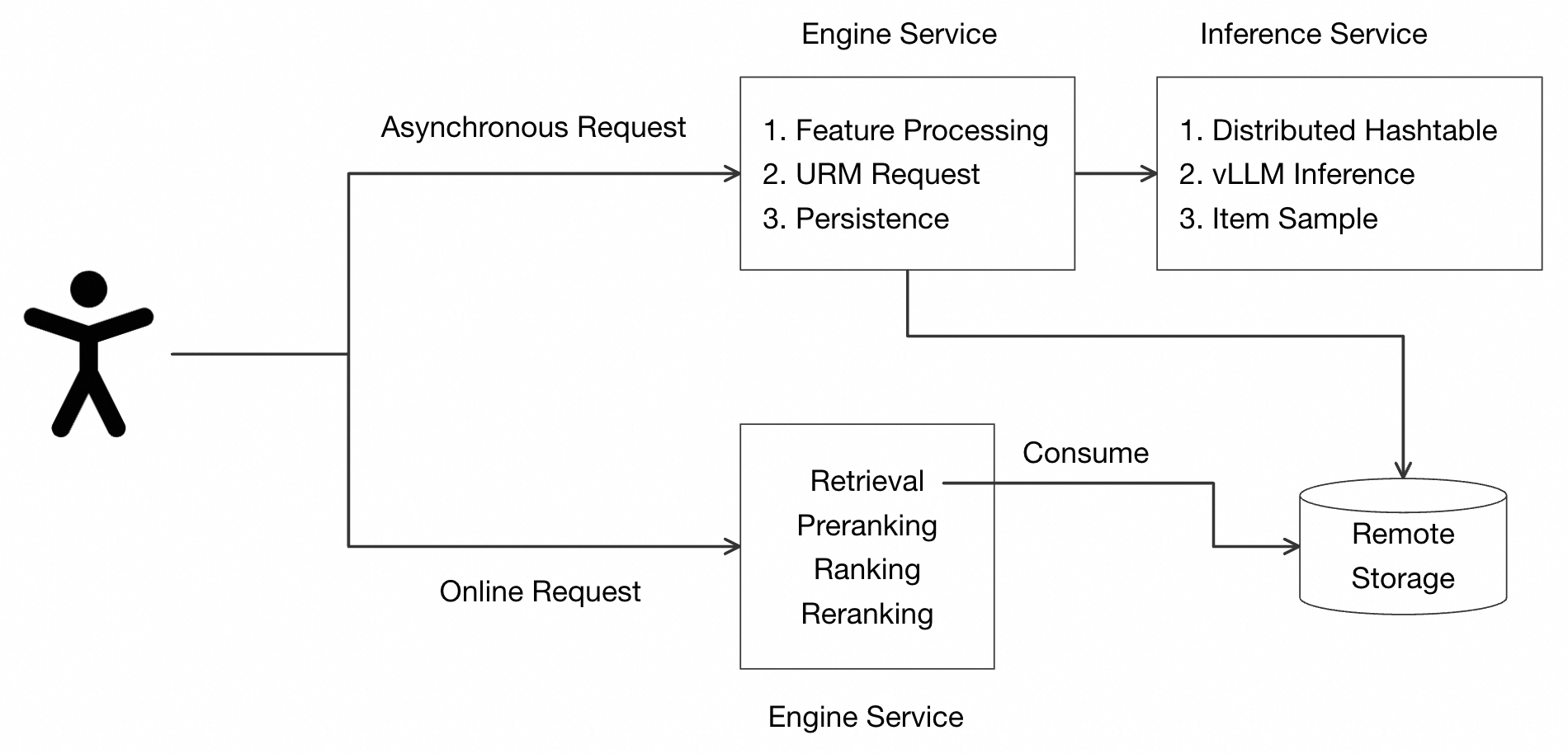
The 7B model has a P99 latency of 233 ms at length 1024, far too slow to run synchronously in an online request. The authors move URM off the request path (the first figure above): a user's clicks, purchases and other actions asynchronously trigger one URM inference, with actions within 10 minutes merged into one trigger; the inference service looks up item vectors, does one vLLM prefill, runs sampling, and writes the result to remote storage. When an online request arrives, the retrieval stage reads that result directly. The authors say this keeps compute cost comparable to ordinary model-based retrieval.
In an online A/B test from April 28 to May 14, 2025, advertising revenue rose 3.01%, CTR 0.78%, CVR 1.24% and the number of long-tail items 2.23%. The authors also note that because the objective can be changed as text, they can A/B different objective sentences and feature combinations online to tune results without retraining.
Limitations as I see them
First, results are not real time. Retrieval results are computed asynchronously after user actions and stored, with actions within 10 minutes merged into one trigger, so what an online request reads can trail the user's latest actions by a few minutes. The abstract's "latency within tens of milliseconds" does not hold for the default 7B model: the appendix table puts its P99 at 233 ms at length 1024. Going online works because the asynchronous design takes inference off the request path, and the authors say plainly that this trades freshness for compute.
Second, training is expensive. On 64 H20 GPUs, Qwen-7B takes 25 hours for 50 million samples. To finish each day's data within 24 hours, the authors sample the training data down to 5% and train one epoch. For teams with large data volumes, this means LLM retrieval learns only a small part of each day's logs.
Third, not every objective improves. URM loses on 3 of the 9 objectives, by the most on long-term interest (0.285 vs 0.337). Pushing exploration up by instruction also drops click retrieval by about 19%. "One model replaces many channels" holds on the aggregate metric, but before replacing any specific channel, check that channel's own metric.
How a recommendation team could try it
- Pick two or three objectives that already have dedicated channels, build URM-style unified retrieval with a smaller LLM (say 1.5B), and compare offline R@K channel by channel to see whether the unified model hurts any of them.
- Raise the number of readout slots from 8 and 32 up to 128 and check whether recall keeps rising; also compare "discriminative + transferable parts" with ID embeddings alone on new items.
- Sweep sampling rounds from 2 to 5, use "recall with sampling ÷ recall with full scoring" to confirm how many rounds suffice, then set the online cost.
- Online, first connect one channel in the asynchronous, store-the-result style, A/B different objective sentences, and check whether revenue, CTR and long-tail share move in the same direction.
Verdict
The key lesson: the value of an LLM in retrieval is not only quality but taking the retrieval objective out of the model architecture and turning it into one input sentence that can be changed at any time.
| Dimension | Assessment |
|---|---|
| Problem importance | High. Maintaining many retrieval channels and cold-starting new objectives is a common burden in recommender systems |
| Novelty | Medium-high. Readout slots, a factorized item table and neighbor sampling are not entirely new, but together they let an LLM produce results over tens of millions of candidates in one forward pass |
| Evidence | Fairly strong. Industrial offline comparisons on 9 objectives, ablations of each part and an online A/B, though URM loses on 3 of the 9 objectives |
| Engineering cost | High. Full fine-tuning of a 7B model, a distributed hashtable, a vLLM inference service and asynchronous result storage all need to be built |
| Worth trying | Yes. Teams with several retrieval channels and frequently changing objectives can first verify offline, with a small model, that unified retrieval does not hurt the main channel |
How did this read for you?
Hoot made a note. Thanks for the feedback.

One tap, no sign-in; tap again to undo. Only anonymous counts are kept, never who you are.
Discussion
Add experiment details, reproduction notes or a different take. Requires a GitHub sign-in.
Loading the discussion…