Contents · 10 sections
1What problem IKE solves2First, what the Isolation Kernel is3How vectors are stored and similarity is computed4Ablation: why dimensions are chosen at random5Experimental setup6Main results: exhaustive search7ANN search and other compression methods8Where the evidence needs discounting9If you want to try it in your own system10Conclusion and assessmentSHARE

IKE (Isolation Kernel Embedding) tackles the problem that LLM text embeddings are too large and too slow to search. It does so without training any model. Models such as LLM2Vec and Qwen3-Embedding-8B output 4096-dimensional float32 vectors, 16 KB per document. IKE builds a few thousand small random trees on the corpus. It replaces each vector with "which leaf it lands in for each tree" and stores only the leaf indices, so a document needs just 1 to 2 KB. On 6 retrieval datasets, memory drops to 1/8 to 1/16. MRR@10 stays at 98% to 101% of the original vectors, which shows the compression barely hurts ranking quality (Table 1). The design that really matters in the ablations is that partitions never look at all dimensions at once: each iForest node picks one random dimension, and each IKE_VD (VD stands for Voronoi diagram partitioning) partition uses a fixed random subset of a few dimensions; the same idea using all dimensions (VDeH) loses half of its nDCG@10 on FiQA2018 (Table 3). My judgment: for teams running vector retrieval, this is a compression scheme that costs almost nothing to try and the evidence is solid, but the comparison lacks the most common scalar quantization, and the speedup on a large corpus is about 6x, far below the peak figure in the abstract.
What problem IKE solves
The cost of vector retrieval comes from two places: each document stores a high-dimensional float vector, and each query computes inner products against many vectors. Among existing compression schemes, MRL requires full retraining of the embedding model to obtain vectors that can be truncated. CSR (Contrastive Sparse Representation) freezes the LLM and trains only an MLP that sparsifies the vector, but each code length needs its own training run, and the mapping itself is a 4096-dimensional matrix multiplication (Sections 1 and 4.3).
IKE's approach involves no learning at all: it builds a random Isolation Forest on the corpus embeddings, uses each tree's leaf index as the new discrete representation, and uses "in how many trees two points land in the same leaf" as the similarity. The authors' other contribution is theoretical. They extend the three criteria for a "good hash" proposed with VDeH to four, the fourth being that partitions must be sufficiently diverse from one another, and they use this criterion to explain why VDeH performs poorly on LLM embeddings (Section 3.3, Appendix C.4).
First, what the Isolation Kernel is
The Isolation Kernel is a data-dependent similarity. It works like this: randomly sample ψ points from the corpus and use some random partitioning to split the space into ψ cells, each containing exactly one sampled point. If two vectors fall in the same cell, this partition counts them as similar once. Repeat t independent random partitions, and the similarity is "the number of times they fall in the same cell divided by t" (Section 2).
The difference from cosine similarity is that the partitions follow the data: cells are small where data is dense and large where it is sparse. So in dense regions two points must be very close to be grouped together, while in sparse regions points somewhat farther apart can still be grouped together.
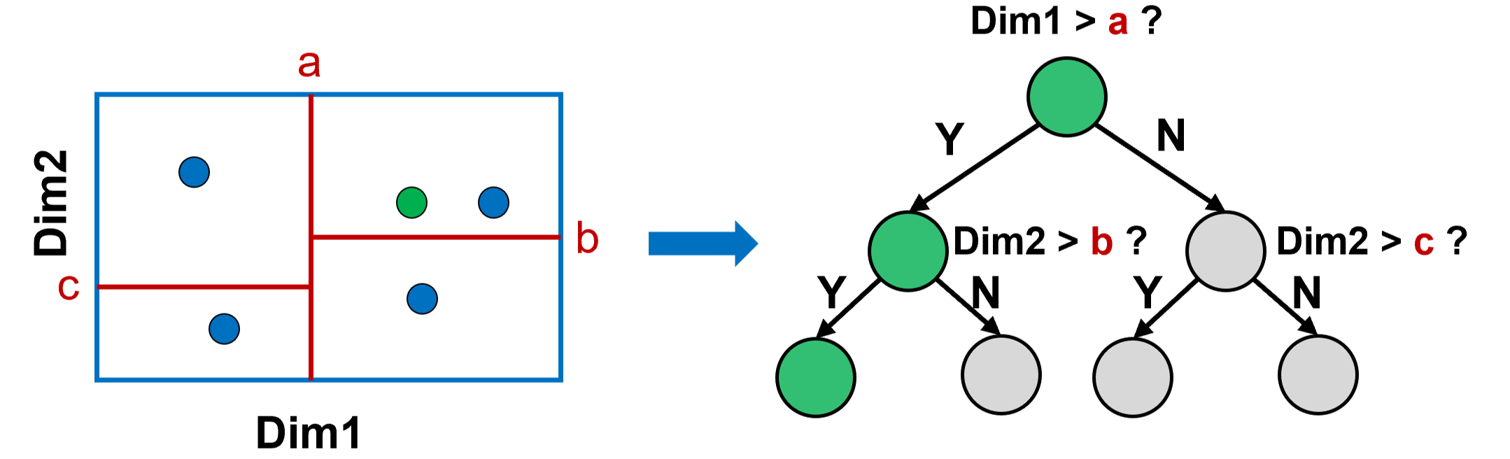
By default IKE uses iForest for partitioning. Each iTree is a binary tree: every internal node picks a random dimension q and a random split value p between the minimum and maximum of the sampled points in that dimension; points greater than p go one way and the rest go the other, and splitting stops when one of three conditions holds: a leaf contains only one sampled point, the tree height reaches the cap ⌈log₂ψ⌉, or the split fails to produce two non-empty subsets (Section 4.1 and the tree-building algorithm in the appendix). So when the cap is reached a leaf may still hold several sampled points, but each tree has at most ψ leaves, and ⌈log₂ψ⌉ bits are enough to store a leaf index. The whole process has no optimization objective, not even a greedy search.
How vectors are stored and similarity is computed
After t trees are built, each vector is represented as t integers, where the i-th integer is the index of the leaf it reaches in the i-th tree, ranging from 1 to ψ. Each index needs only ⌈log₂ψ⌉ bits, so a document takes t·⌈log₂ψ⌉ bits. By default t equals the original dimension 4096. With ψ=12 each index is 4 bits and a document is 2 KB, exactly 1/8 of the float32 vector; with ψ=3 each index is 2 bits, a compression to 1/16 (Section 3.1, Table 1).
At query time, the query vector is first mapped through the same trees into t leaf indices, then the system counts how many indices it shares with each document. This counting is written as bit operations: first XOR the two codes, so the segment for a matching index is all zeros. Then shifts and OR fold the differences within each index into the lowest bit of its segment, so a 0 in that bit means the index matches. Next a mask sets all other bits to 1, popcount counts the 1 bits, and subtracting that count from the total number of bits gives the number of matching indices (Section 3.2). To keep codes byte-aligned, the implementation uses only 1, 2, 4 or 8 bits per index (Section 3.2). Under this restriction, when ⌈log₂ψ⌉ is 3 (for example ψ=5 or 8) the index can only be padded to 4 bits, and the storage formula above should use the padded width; the ψ=3 and ψ=12 used in Table 1 are exactly 2 and 4 bits and are unaffected. With ψ=2 each index is a single bit and this reduces to ordinary Hamming distance.
Mapping a query only needs ⌈log₂ψ⌉ comparisons per tree, with complexity O(t⌈log₂ψ⌉); CSR's mapping goes through a 4096-dimensional MLP layer, on the order of O(d²) (Section 4.3). This is the main reason IKE is an order of magnitude faster than CSR later on.
The trees are built independently, so the code length can be adjusted afterwards: keeping only a subset of the trees gives a shorter code without retraining anything (Section 3.1). This serves the same purpose as MRL's truncatable embeddings, but without retraining the LLM.
Ablation: why dimensions are chosen at random
IKE's predecessor VDeH partitions with a Voronoi diagram: sample ψ points as centers and assign each vector to the nearest center, with distance computed over all 4096 dimensions. The authors found that VDeH performs badly on LLM embeddings, so they built a generalized version IKE_VD: each partition first draws m random dimensions and fixes them, and that partition's centers, document codes and query codes all compute distance over only those m dimensions; when m equals all dimensions it is VDeH (Section 2, Appendix D).
Figure 2 shows nDCG@10 on FiQA2018 as m goes from 1 to 4096. For m between 1 and a dozen or so, both embeddings stay close to the original-vector baseline. The larger m gets, the more it drops. At m=4096, i.e. VDeH, LLM2Vec falls from the low 50s to about 26. This shows the problem lies in "every partition looks at all dimensions": although each partition draws new random centers, all of them use the same distance, so the cells they produce are highly correlated and adding more partitions brings only limited gains (Appendix C.4). The authors summarize this as the fourth criterion, that partitions must be diverse (Appendix C.4). iForest looks at only one random dimension per node and satisfies this naturally.
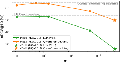
Table 3 puts the implementations side by side:
| Implementation (FiQA2018) | LLM2Vec MRR@10 | LLM2Vec nDCG@10 | Qwen3 MRR@10 | Qwen3 nDCG@10 |
|---|---|---|---|---|
| IKE (iForest) | 60.13 | 52.58 | 71.14 | 63.25 |
| IKE_VD, best m | 60.23 | 52.89 | 71.99 | 64.03 |
| IKE_VD, m=1 | 59.76 | 52.61 | 69.87 | 62.16 |
| VDeH (m = all dimensions) | 32.07 | 25.84 | 58.91 | 49.78 |
IKE_VD with a tuned m is slightly better than the iForest version, but the authors still recommend iForest, because IKE_VD adds a hyperparameter m and its mapping computes ψ distances of m dimensions, with complexity O(mtψ), more expensive than walking a tree (Section 4.5.3). I agree with this trade-off; a gap of 0.3 to 0.8 points is not worth one more parameter to tune.
Experimental setup
The datasets are HotpotQA, FiQA2018, FEVER-HN and Touche2020.V3 from MTEB. Istella22 and TREC DL 23, which have graded relevance labels, are added (Section 4.1, Appendix Table 4). HotpotQA has 5.23 million documents and is the only corpus above the million scale, so it best shows behavior at scale. The embedding models are LLM2Vec (Mistral-7B backbone) and Qwen3-Embedding-8B. By default t equals the original dimension, and ψ is grid-searched per dataset on a validation set (Appendix E.2). Touche2020.V3 has no official validation set, so the authors randomly take 30% of the test set for tuning and evaluate on the remaining 70%. Experiments run on a CPU server with two Xeon Gold 6330 processors (56 physical cores), and exhaustive search over the original vectors uses Faiss (Section 4).
Main results: exhaustive search
| Dataset (LLM2Vec) | Memory | Search time (s) | MRR@10 | nDCG@10 |
|---|---|---|---|---|
| HotpotQA original vectors | — | 326.61 | 83.83 | 74.09 |
| HotpotQA IKE (ψ=12) | 1/8 | 54.82 | 83.69 | 73.24 |
| Istella22 original vectors | — | 1.56 | 68.11 | 63.88 |
| Istella22 IKE (ψ=16) | 1/8 | 0.62 | 68.92 | 63.86 |
| TREC DL 23 original vectors | — | 0.90 | 97.56 | 73.10 |
| TREC DL 23 IKE (ψ=3) | 1/16 | 0.16 | 98.11 | 71.78 |
The numbers come from Table 1, and search time is the total over all queries. On the largest dataset, HotpotQA, search time shrinks to about 1/6 and MRR@10 is only 0.14 points lower, which shows that compression is nearly lossless on a 5-million-document corpus. IKE's tree building plus mapping time is also shorter than building the Faiss index over the original vectors (Table 1), so offline cost will not be an obstacle.
The highest speedup of "16.7x" appears on Touche2020.V3 (Qwen3), a small corpus of a few hundred thousand documents, where search time drops from 1.59 s to 0.095 s; in the same row nDCG@10 falls from 76.41 to 73.35, a 3-point loss and the largest in Table 1. On the largest corpus, HotpotQA, the speedup is 6.0x (LLM2Vec) and 5.8x (Qwen3), so the "up to 16.7x" in the abstract should be expected to be about 6x in practice.
ANN search and other compression methods
Production systems usually do not run exhaustive search but use HNSW or IVF indexes. IKE plugs into HNSW directly: graph building and search follow the original algorithm, with cosine similarity replaced by IKE's "number of shared leaves" (Appendix F.1). IVF still uses the original vectors for k-means clustering and for finding the nearest clusters, and IKE scores only within clusters.
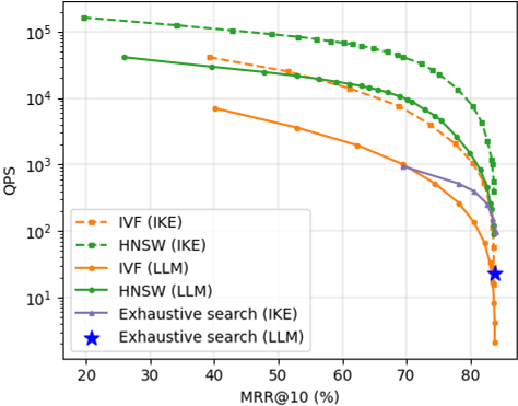
In Figure 4, at the same MRR@10 of about 61%, HNSW QPS rises from 16,000 with the original vectors to 64,000 with IKE; the gain for IVF is about 6 to 8x (Section 4.2). This means IKE does not only speed up exhaustive search; it also holds when plugged into an existing graph index.
The comparison against CSR (Figure 5) is done at fixed code lengths. Each CSR sparse vector keeps k non-zero values and its code length is counted as 4k bytes, while IKE matches the same code length by adjusting t and ψ; for example, at 128 bytes IKE uses t=1024 and ψ=2. These code lengths are all much shorter than the 2 KB in Table 1, so on HotpotQA IKE's exhaustive search takes 4 to 12 seconds rather than the 54.82 seconds of Table 1. At the same code lengths CSR needs 104 to 237 seconds, and IKE has comparable or higher nDCG@10 (Section 4.3). This search time includes query mapping, whereas the original CSR paper counted only the similarity computation (Section 4.3). MRL was not compared because it requires full retraining and the authors lacked the compute.
Against other training-free compression methods (Figure 6, fixed code length), at a 512-byte code and nDCG@10 around 60%, HNSW (IKE) reaches about 2.9 times the QPS of IVF (PQfs); at 1024 bytes and nDCG@10 around 70%, about 10 times that of IVF (rpLSH) (Section 4.4). rpLSH is the classic hash that takes sign bits after random hyperplane projections, and PQfs is fast-scan product quantization in Faiss. This means that under the same storage budget, IKE's codes are more useful than these two classic compressed codes.
Where the evidence needs discounting
The comparison lacks the most common schemes. The most common industrial way to compress vectors is int8 scalar quantization, or simply taking sign bits for binarization, and neither needs training. rpLSH and PQfs partly cover this family, but I would rather see IKE against int8 at the same memory, because int8 compresses only to 1/4 with almost no loss in accuracy and is the default choice for many teams.
ψ is tuned per dataset on a validation set, and the Touche2020.V3 validation set comes from 30% of the test set. This does not cross a methodological line, but it means ψ has to be tuned once per corpus. Table 2 shows that as ψ goes from 2 to 16, nDCG@10 on Istella22 only moves between 75.71 and 76.35, so the effect is small, which is somewhat reassuring.
The trees are built on a fixed corpus. New documents can be mapped with the old trees directly, but if the corpus distribution drifts, whether the old partitions remain suitable is a case the experiments do not cover. The limitation the authors acknowledge themselves is that cross-modal retrieval works less well, possibly because of the modality gap between image and text embeddings (Limitations section).
If you want to try it in your own system
The cost is low. Sample from your existing corpus embeddings to build t=4096 iTrees, start ψ at a few settings such as 2, 4, 8 and 16, map both documents and queries into leaf indices, and compare recall@100 and QPS against your current float32 or int8 index on an offline evaluation set. With ψ=2 the code is an ordinary binary code, so existing Hamming-distance retrieval code can be reused directly. If memory is the bottleneck, also try keeping only a subset of the trees and look at the curve of code length against recall, without retraining the embedding model.
Conclusion and assessment
IKE's advance is that it turns LLM embeddings into short discrete codes with a random iForest, with no training and an adjustable code length, and it explains VDeH's failure with the criterion that partitions must be diverse; the large gap between VDeH and IKE in Table 3 directly supports that explanation. The main results hold across 6 datasets and 2 embedding models, and they also hold with HNSW.
What needs discounting is the size of the speedup: about 6x on a large corpus, not 16.7x, and the comparison lacks int8, the most practical competitor. I would treat it as a candidate for compressing vector retrieval and test it side by side with int8 and binary quantization on my own corpus before deciding.
How did this read for you?
Hoot made a note. Thanks for the feedback.

One tap, no sign-in; tap again to undo. Only anonymous counts are kept, never who you are.
Discussion
Add experiment details, reproduction notes or a different take. Requires a GitHub sign-in.
Loading the discussion…