Contents · 9 sections
1What problem is it really solving?2The pipeline: prediction is one link in the routing chain3Why predict log throughput, and why bin it?4The most useful feature: how fast this job ran before5How well does it work?6Which changes actually raised accuracy?7Limitations as I see them8How a training platform team could try it9VerdictSHARE

The same training job can often run on several accelerator types, and which one is cheapest depends on its throughput on each. A job placed on the wrong type still finishes without any error, so the extra cost goes unnoticed. LEAP, a hardware-selection service the authors run in a production fleet, predicts a job's throughput on every candidate type at submission time, then ranks the types by predicted throughput per unit cost, choosing hardware for tens of thousands of training jobs a day. 77% of its predictions land within 20% of the measured throughput. After six months it ranked 95% of the eligible training GPU-hours, and the authors estimate it saves about 3% of training compute cost. Teams running mixed accelerator fleets should read it: it turns the invisible waste of a job on the wrong hardware into a measurable prediction problem, and reports which features actually improve accuracy.
What problem is it really solving?
Take an illustrative case. A ranking-model training job needs 64 machines, and two accelerator types in the fleet can run it.
| Candidate (illustrative) | Cost per hour | Predicted throughput (samples/s) | Throughput per unit cost |
|---|---|---|---|
| Type A | 1.0 | 1,000 | 1,000 |
| Type B | 1.6 | 1,800 | 1,125 |
Type B is pricier, but this job gets 80% more throughput on it, more than the 60% price gap, so per unit cost B wins. A job with heavier communication or a smaller batch could flip the answer. The hard part is filling in this table before the job has run, across more than twenty hardware types.
The fleet in the paper runs about 25,000 training job attempts a day from about 660 model types. The distribution is long-tailed: on the day the paper shows, the 560 least common model types together account for 22% of attempts. A rule built only for the common models leaves a large share of the work unserved.
The old method was a lookup table keyed on model type, trainer count (the number of hosts the job uses), batch size and hardware type. It failed in two ways. First, these four values do not pin down throughput: for 56% of attempts, the 10th and 90th percentile throughput under the same key differ by more than 1.5 times, so no single prediction can land within 20% for all of them. Second, the table covered only 19 model types and returned a value for 13% of attempts on a held-out day.
The pipeline: prediction is one link in the routing chain
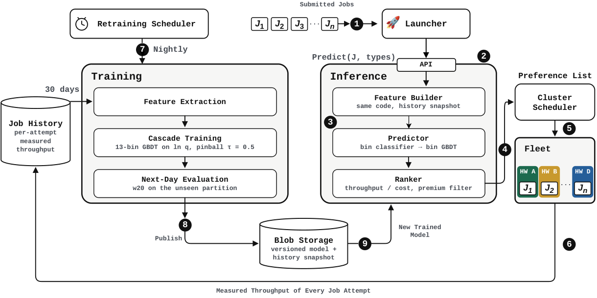
The chain has three stages, and LEAP owns only the middle one:
- The job launcher decides which hardware types can host the job.
- LEAP builds one feature row per candidate type: the job configuration as submitted, plus that type's hardware specifications and the job's history features. It then predicts throughput, divides it by the job's cost on that type to get a score, and sorts the types by score into a preference list.
- The cluster scheduler treats the list as a preference, not a hard constraint, and places the job according to free capacity.
Two engineering choices keep it cheap and safe. The prediction library is linked into the launcher, so a routing call is a function call rather than a network request. Any failure, such as an empty candidate set, a missing feature or a model file that will not load, returns an empty list, and the scheduler places the job as if LEAP did not exist. At worst, a LEAP problem falls back to the old behavior.
Why predict log throughput, and why bin it?
Throughput spans a huge range. In one day of 22,495 rows, measured throughput runs from single digits to over a million, seven orders of magnitude. Even on a single hardware type, the 95th and 5th percentiles differ by 42 to 701 times. A regressor on raw throughput is dominated by the largest jobs.
So LEAP predicts the logarithm of throughput with a pinball loss at the median, which equals half the absolute error in log space. Exponentiating gives the conditional median of throughput.
A single regressor still fits the extremes poorly. LEAP splits jobs into 13 throughput bins and trains one gradient-boosted regressor per bin, each responsible for its own range: Hoot says

Use the arrows to see four steps. Step 2's numbers are illustrative. The point: training groups rows using true throughput, but online only the classifier's guess picks the group, and a wrong guess sends the job to an ill-fitting regressor. Source: paper §2.2 training and serving equations: 13 equal-frequency bins, at most 3 alternations, early stop below 2% moved, the bin classifier picks from features
- Split the training rows into 13 equal-frequency bins by log throughput and fit one regressor per bin.
- Reassign every row to the regressor that predicts it best, then refit. Alternate at most three times, stopping early when fewer than 2% of rows change bin.
- Finally train a classifier that assigns a row to a bin from its features alone. At serving time the true throughput is unknown, so this classifier picks the regressor.
An illustrative example: a small job runs at 50 samples per second and a large one at 500,000. The classifier first decides which bin each belongs to, and the exact number comes from the regressor that specializes in that range. In practice it must pick one of 13 groups: the classifier learns which regressor each row was finally assigned to after the reassignment. When it picks the wrong one, a regressor that does not fit this row answers.
In the ablation below, this binned cascade adds only 0.5 points. The authors themselves say that single-day differences of one or two points are within night-to-night variation. So the clear gains come from the architecture features and the deeper trees described later; binning is a small extra.
The most useful feature: how fast this job ran before
Whether a job has run before, and how fast, is the signal the trained model leans on most. For each job family LEAP keeps the previous log throughput, the running mean and standard deviation, the number of prior runs, and the days since the last one. To avoid an extra lookup by job name when the job launches, each training run packs a snapshot for up to 250,000 job families into the published model. Families are matched by job name with run-specific identifiers stripped. Online, only the days since the last run are recomputed. Jobs missing from the snapshot are cold starts and get an explicit default value rather than zero.
Shuffling one feature at a time and measuring the accuracy drop, the mean prior log throughput comes first at 36.7 points, followed by trainer count and batch size. Hardware specifications account for only 5.8% of total importance. The authors note this understates hardware: the specifications move together, so shuffling one leaves the others carrying the same information. For the same reason, this ranking shows how much the model relies on a feature, not how much would be lost without it. In the ablation below, adding history features gives only 2.5 points. The authors explain that a model retrained without history features can recover part of the same signal from correlated inputs such as job scale.
How well does it work?
First, a head-to-head with the old table. On a held-out subset of one day (7,131 jobs from 276 model types), the table returned a value for 946 and LEAP for all of them. On those 946 jobs only (numbers from Table 1 of the paper):
| Method | Within 10% | Within 15% | Within 20% | Median predicted/measured |
|---|---|---|---|---|
| Lookup table | 33.4% | 45.0% | 53.2% | 1.11 |
| LEAP | 72.1% | 80.6% | 85.1% | 1.00 |
These 946 jobs belong to the models the table was built for, and LEAP is still more than 30 points ahead. So the old method's problem was not only coverage: its key simply does not determine throughput.
Second, the long run. Over 30 consecutive nightly retrains, each scored on the day after its training window, the median share within 20% is 77.0%, ranging from 73.5% on the worst night to 80.6% on the best. Nights differ by several points, so a single day can mislead, which is why the authors use the 30-night median as the headline.
Tighter tolerances still hold up. On a separate held-out day used for model comparisons, 68.9% of predictions were within 10% and the median error was 6.9%, so most predictions are fairly close.
Third, deployment impact. In the first half of 2026, the share of eligible training GPU-hours that received a LEAP ranking grew from 58% to 95%. Being ranked is not the same as running on the top pick: in six days in August, only 19.9% of jobs and 30.0% of GPU-hours ran on the top-ranked type, because the scheduler must respect capacity. Jobs LEAP can route make up about half of the fleet's training cost, and the authors estimate an overall saving of about 3%.
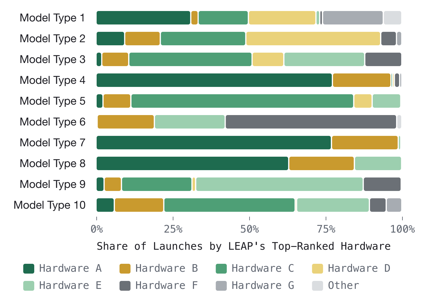
This figure shows why a fixed rule fails. Different launches of the same model differ in trainer count, batch size and eligible types, so the best-value type changes too. Model Type 1 in the paper had 5,527 launches in a week, and four hardware types were each ranked first in 16% to 31% of them.
Which changes actually raised accuracy?
On one fixed held-out day, the authors start from a plain gradient-boosted tree and add changes one at a time (this day is easier than average, so its values sit above the 77% headline and only the differences matter):
| Configuration (cumulative) | Within 20% |
|---|---|
| Gradient-boosted tree baseline | 72.3% |
| + job-history features | 74.8% |
| + ratio features computed from the configuration | 76.6% |
| + architecture features | 80.7% |
| + deeper histogram GBDT | 82.8% |
| + 13-bin cascade | 83.3% |
The ratio features multiply or divide configuration values known at submission, such as the total batch size across all trainers and the ratio of data readers to trainers, so they need no measured throughput. The biggest gain came from architecture features, 44 summary values extracted from the model definition such as layer counts, worth 4.1 points. The 13-bin cascade added 0.5 points.
No other model family won. LightGBM reached 69.4%. The closest was TabPFN v2 (a transformer pretrained on synthetic tabular data that predicts from similar examples given in context) at 79.1%, but it needs a GPU and a retrieval step at serving time. Fine-tuning Gemma 3 27B to output throughput as text reached 69.0%, and a LoRA-tuned Llama 4 only 50.8%. Writing the job configuration as text, encoding it with Qwen3-Embedding and adding a small network gave, at best, 3.7 points less than the cascade (compared on another held-out day). The authors' likely explanation: text tokens do not keep the magnitude of numbers, and throughput depends mostly on numbers such as trainer count and batch size.
The only match was a graph neural network over the computation graph (the authors' reimplementation of DNNPerf). This comparison uses a different setup: on the same jobs from three other evaluation days, averaged over 10 random seeds, both it and the cascade reach 77.4%. But it needs a GPU at serving time and a graph cache of about 400 GB, and the graph itself added only 0.25 points. For a routing service called tens of thousands of times a day, that cost is not worth it.
Limitations as I see them
First, new hardware cannot cold-start. The authors ran the hold-out test on the graph-based comparison model: leaving one hardware type out of training cost 37 points, while removing the same number of random rows cost 1.7. The paper says the cascade does not extrapolate to new types either. A new type has to run real jobs first, and LEAP ranks it after the next nightly retrain.
Second, new model families suffer too. Holding out one family cost the cascade 49.7 points and the graph model 37.0, likely because the classifier has no basis for putting an unseen family into the right throughput bin.
Third, both headline numbers need a discount. The 77% is averaged over job attempts, not weighted by GPU-hours, so the few large jobs that consume most GPU-hours carry little weight in it. The 3% saving is an estimate, and only 19.9% of jobs actually ran on the top-ranked type: however accurate the prediction, a job cannot move when the better type is full.
How a training platform team could try it
- Measure the waste first: from historical throughput of similar jobs on different types, compare the best-value type with the type actually used. If the gap is small, skip the project.
- Start simple: a gradient-boosted tree predicting log throughput from job configuration, hardware specifications and the job's own past throughput. Evaluate with the share of predictions within 20% of measured throughput, scored only on days after the training window. The authors report that an early evaluation inside the training window overstated accuracy by more than 20 points.
- Hand the ranking to the scheduler as a preference only, and return an empty list on any failure. That keeps rollout risk low and lets you enable it one model type at a time.
- If there is room, add architecture features first; the binned cascade is optional. Before a new hardware type enters routing, run a small set of representative jobs on it, which the authors propose as future work.
Verdict
The key lesson: the hard part of hardware selection is not a fancy model but a reliable throughput estimate before the job runs, and that estimate comes mainly from the job's own history, scale and architecture.
| Dimension | Assessment |
|---|---|
| Importance | High. Routable jobs are about half of training cost, and wrong placement raises no error, so the waste goes unseen |
| Novelty | Medium. The core is gradient-boosted trees with a binned cascade; the value is running it as a service called tens of thousands of times a day |
| Evidence | Fairly strong. 30-night rolling evaluation, a head-to-head with the old table, and ablations across model families; the 3% saving is an estimate |
| Engineering cost | Low to medium. CPU-only inference inside the launcher; the main investment is the feature table and nightly retraining |
| Worth trying | Yes for training platforms with several hardware types and jobs that can move between them |
How did this read for you?
Hoot made a note. Thanks for the feedback.

One tap, no sign-in; tap again to undo. Only anonymous counts are kept, never who you are.
Discussion
Add experiment details, reproduction notes or a different take. Requires a GitHub sign-in.
Loading the discussion…