SHARE

To make a generative recommender stronger, teams usually add layers, which means adding parameters and memory. Tencent's LoopGR (a generative recommendation backbone that reuses one decoder in a loop) takes another route. It runs the same decoder several times, and between passes a very small GRU module rewrites the representation of the user's history based on the decoder's current prediction state, then hands it to the next pass. Computational depth is thus decoupled from parameter count. At the same budget of about 0.5 GFLOPs, it uses only 1.3M parameters and still beats a 2.7M-parameter encoder-decoder. On Tencent's industrial data its Recall@10 is 0.6458, above TIGER's 0.6125 and the production model BARGE's 0.6277. To control latency, the authors distill the 16-loop model into a 4-loop one, cutting single-request latency from 211 ms to 50 ms with almost no loss in quality.
Teams that care about the serving cost of generative recommendation should read this. It answers a practical question: when the parameter and memory budget is fixed, where else can quality come from? The core idea in one sentence: the decoder keeps revising its prediction of the target SID, and the updater makes the user history change along with that prediction. The evidence comes mostly from small datasets with ten to sixty thousand items and models at the million-parameter scale, and there is no online A/B on the industrial data, which limits how far the conclusions can be pushed.
What problem is it actually solving?
SID-based generative recommendation encodes each item as a few levels of discrete tokens. The model reads the user's history and generates the SID of the next item level by level. Compute is spent in two places: understanding the history and generating the target SID. Existing backbones split this differently.
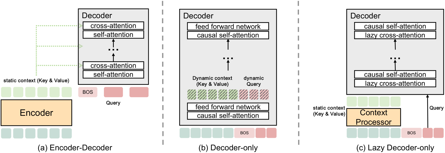
All three share one property: once the history is encoded, it stays fixed during generation. An illustrative scenario shows why this matters:
| User history (illustrative) | When decoding the first SID level | How the history ideally should change |
|---|---|---|
| running shoes, protein powder, yoga mat, children's picture book | first-level prediction leans to "sports" | shoes and protein powder should gain weight, the picture book should lose it |
| same | model with a fixed history | all four items keep the same representation, and the second level must still pick from a mixed history |
The other problem is that depth is tied to parameters. To refine the history a few more times, you need more layers, and recommender memory and latency budgets are far tighter than those of large language models. LoopGR tries to solve both: let the history evolve during generation, and add rounds of compute without adding parameters.
Overall structure: one encoder, one shared decoder, one small updater
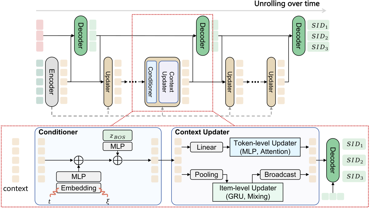
| Component | What it does | How many times it runs |
|---|---|---|
| Encoder | encodes the SID tokens of every history item into the initial history representation | once |
| Decoder | reads the current history and its own hidden state from the previous pass, and predicts the next SID token | for every SID level, one loop: one pass in each of rounds, plus one final pass, all sharing parameters |
| Updater | rewrites the history using the decoder's current state | times after each decoding pass, sharing parameters |
The authors call the decoder loop the high-level cycle, with count , and the updater loop the low-level cycle, with count . The whole flow is: encode once, then treat "decode once, update times" as one round, repeat it times, and finally decode once more on the rewritten history. For example, with and the order is encode, decode, update, decode, update, decode, so the decoder runs 3 times and the updater twice.
The updater: letting the history follow the prediction
Why is an updater needed? If the history stays the same between passes, every decoding pass reads the same history, and repeated decoding can correct very little. The authors tested this: replacing the updater with an identity that does nothing lowers quality by about 8% on average. So the gain comes mainly from the history changing, not from the decoder simply running more times.
The updater rewrites the current history representation, one vector per history SID token. It reads two extra signals. The first is the hidden state at the decoder's BOS position. The BOS position reads the whole history through cross-attention and inherits the state of the previous pass, so the authors use it as the model's overall judgement of the target item; an MLP turns it into a query vector. The second is the current high-level round, low-level round and SID level, turned into a condition vector by an embedding and an MLP. Both vectors are added to every history position. The updater then pools the tokens of each item into one item vector, runs a light GRU along the item order, and broadcasts the result back to the tokens.
The nesting matters. The target SID is still generated level by level. For each level the whole loop runs first, its final prediction fixes that level's token, and the model moves on to the next level with the generated prefix. Inside the loop, each decoding pass takes the hidden states it produced in the previous pass (BOS plus prefix positions) plus the round vector, so the prediction is revised pass after pass rather than recomputed from scratch.
One detail is key: after each rewrite, the result is added back to the original history representation and normalized. Every round is a correction on the original history, not a drift away from the previous round. This anchor makes multi-round loops easier to train.
Walk through the illustrative example. After the first pass the BOS state leans to "sports". The updater reads it and makes the shoes and protein powder stand out. The second pass continues from its previous state on this new history, and the first-level SID distribution becomes sharper. This per-item change is an illustration of the mechanism.
The authors also compared updaters: the default GRU; token mixing, an MLP that blends vectors along the sequence; linear attention; and vanilla attention. All four perform similarly, and token mixing is even slightly better on Sports, so what matters is having a module that rewrites the history, not which operator it uses.
What each loop level does
The authors fix both encoder and decoder to one layer and vary only and .
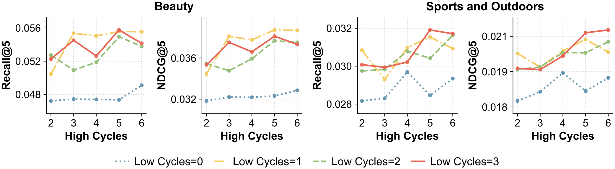
Removing the low-level loop, , clearly hurts; one or two updates bring Recall@5 and NDCG@5 back. Larger generally helps but stops rising monotonically at greater depths. On the larger Sports set, deepening both gives more. The two levels therefore have clear jobs: the high level revises the prediction repeatedly, and the low level adjusts the history between revisions.
The parameter-efficiency comparison is direct. At about 0.5 GFLOPs, LoopGR uses 1.3M parameters against 2.7M for the encoder-decoder, with higher NDCG@5. That pair is the "up to 52% fewer parameters" in the abstract.
Recurrent trajectory self-distillation: from 16 passes to 4
Loops add no parameters but do add latency, because passes run in sequence. The 16-loop model needs 211 ms per request, too slow for serving. The authors' fix is RTSD (recurrent trajectory self-distillation). They train a teacher with all 16 passes, initialize a 4- or 8-pass student from the teacher's weights, and make the student imitate the teacher's whole prediction trajectory.
Why not just take the output after pass 4? The authors tried common ways to save compute: supervising every pass, a gated early exit, and ILSD, the intra-loop self-distillation of Goyal et al. (2026), where shallower loops of the same model imitate deeper ones. Averaged over 8 metrics, they fall 9.7%, 13.2% and 9.4% below the full-budget model; RTSD falls only 3.2%. The authors explain that supervising every pass makes intermediate representations stall early, so later passes barely change and the loop budget is wasted.
The RTSD loss has two terms. The first aligns the student's distribution at each pass with the teacher's distribution at the matching pass, where student pass maps to teacher pass :
Here is the predicted distribution for SID level at a given pass. With a 16-pass teacher and a 4-pass student, : student pass 1 matches teacher pass 4 and student pass 4 matches teacher pass 16, so each student step stands for four teacher steps. Pass means the decoding after round of updates, so pass is the final output, and the student's final distribution is pulled toward the teacher's final distribution. The second term aligns direction: the change in log-probabilities between two consecutive student passes should point the same way as the change between the matching teacher passes, measured by cosine distance. The first term says where each step should land; the second says which way it should move. Hoot says

Term one, L_Traj: where each pass lands
- matching
- student pass 1 ↔ teacher pass 4
- teacher
- (0.6, 0.3, 0.1)
- student
- (0.5, 0.3, 0.2)
- KL(teacher ‖ student)
- ≈ 0.04, pushes code 1 up
It only constrains the distributions at the 4 matched points, not how the student gets between them.
Term two: which way consecutive passes move
- teacher pass 4 → 8
- log-prob change (+0.6, −0.2, −0.4)
- student A pass 1 → 2
- (+0.3, −0.1, −0.2): cosine 1, distance 0
- student B
- (+0.6, −0.4, −0.2): cosine ≈ 0.93, distance 0.07
- student C
- (−0.3, +0.1, +0.2): cosine −1, distance 2
A moves only half as far as the teacher but in the same direction, so no penalty; C moves the opposite way and gets the largest one.
Only 3 candidate codes of one SID level; the distributions and changes are illustrative. The mapping student pass s ↔ teacher pass 4s is from the text (16-pass teacher, 4-pass student). The two examples are independent. That cosine ignores step size is a property of cosine distance that the paper does not spell out, and term one only constrains step size indirectly, through the distributions at matched passes. Source: paper, RTSD: L_Traj averages the KL between each student pass and its matched teacher pass (a(s) = ⌈s·T_tr/T_stu⌉); term two aligns the change in log-probabilities between consecutive student passes with the teacher's matching change, measured by cosine distance
| Model | GFLOPs | Latency (ms) | Sports NDCG@10 | Beauty NDCG@10 |
|---|---|---|---|---|
| teacher, 16 passes | 17.408 | 211.08 | 0.0248 | 0.0448 |
| RTSD student, 8 passes | 8.415 | 104.01 | 0.0250 | 0.0453 |
| RTSD student, 4 passes | 3.918 | 49.82 | 0.0261 | 0.0450 |
The 4-pass student runs at about a quarter of the latency, beats the teacher on all four Sports metrics and ties it on Beauty. Projecting the students' intermediate states to 2D, the authors find the student does not just cut the teacher's trajectory short: it takes one large step in the first pass and then converges in small steps to an endpoint near the teacher's.
Comparison with existing methods
The public data are the Beauty, Sports and CDs (music CDs and vinyl) categories of Amazon 2014. Baselines include classic sequential recommenders such as SASRec and generative recommenders TIGER and HSTU, plus ActionPiece and RPG, which improve the item encoding. The industrial data come from Tencent's production recommender, with TIGER, a lazy decoder-only model modeled on OneRec V2, and BARGE, a generative model in production at Tencent.
| Data | Metric | TIGER | strongest baseline | LoopGR |
|---|---|---|---|---|
| Beauty | NDCG@10 | 0.0384 | 0.0464 (RPG) | 0.0465 |
| Sports | NDCG@10 | 0.0225 | 0.0264 (ActionPiece) | 0.0275 |
| CDs | NDCG@10 | 0.0411 | 0.0451 (ActionPiece) | 0.0447 |
| industrial | Recall@10 | 0.6125 | 0.6277 (BARGE) | 0.6458 |
| industrial | Recall@100 | 0.7164 | 0.7496 (BARGE) | 0.7675 |
On public data LoopGR is best on 8 of 12 metrics and slightly behind ActionPiece on CDs. Since it uses plain RQ-VAE codes rather than a specially designed SID, this suggests the gain comes from the backbone itself. On industrial data it leads everywhere, and its margin over TIGER grows with the cutoff, which means the loop mainly helps recall deeper in the list.
Limitations as I see them
First, the public data are small. Beauty has about 12,000 items and an average history of 8.88, and the models have only millions of parameters. Halving parameters at this scale means something very different from industrial models with billions of parameters, and the paper's evidence does not reach the question of whether the loop keeps its parameter efficiency at that size.
Second, read the industrial result with care. The best industrial variant uses token mixing as the updater, and Table 2 reports that variant, while the public main results use the GRU; the updater appears to have been chosen on the same industrial data. And there is only offline recall, no online A/B.
Third, latency is still high. Even at 4 passes a request takes about 50 ms, measured at batch size 1, and the loop is inherently sequential, so it cannot be amortized by parallelism the way a wider network can.
How a recommendation or search team could try it
- Start with the cheapest control: on an existing SID generative model, make the decoder share parameters and loop 2 to 3 times without an updater. Per the paper the gain is limited, which makes it a good baseline.
- Add the updater, rewriting the history from the BOS state and keeping the anchor back to the original history. If this clearly beats step 1, "history follows prediction" holds on your data.
- Train a teacher with many loops, distill it with RTSD into a 2- to 4-pass student, and compare latency and metrics. Compare against per-pass supervision to confirm distillation beats simple truncation.
- Finally run an A/B where parameters are constrained, such as a memory-bound retrieval service, comparing against the current backbone at equal parameter count.
Verdict
In recommender systems bound by parameters and memory, trading loops for depth is a viable path, and the key is to update the user history along with the prediction inside the loop rather than letting the decoder spin on a fixed input.
| Dimension | Assessment |
|---|---|
| Problem importance | Medium-high. Recommender parameter and memory budgets are tighter than LLMs', so compute allocation is a real problem |
| Method novelty | Medium-high. Looped Transformers are not new; the novelty is rewriting history between decoding rounds and distilling along the trajectory |
| Experimental evidence | Medium. Ablations and depth analysis are complete, but public data are small and industrial results are offline only |
| Engineering cost | Medium. Few parameters, but sequential loops add latency and require distillation |
| Worth trying | Worth trying for memory-bound generative retrieval, starting with the updater control |
| Fit | SID generative recommendation with tight parameter budgets that can accept generation latency of tens of milliseconds |
How did this read for you?
Hoot made a note. Thanks for the feedback.

One tap, no sign-in; tap again to undo. Only anonymous counts are kept, never who you are.
Discussion
Add experiment details, reproduction notes or a different take. Requires a GitHub sign-in.
Loading the discussion…