Contents · 10 sections
1What problem is it solving?2The overall pipeline3Per-stage recomputation: small-memory GPUs compute twice, large-memory GPUs do not4The combined score: any term that grows is penalized5How do tens of thousands of configurations become affordable to search?6Experiments: is the prediction accurate, is the ranking right?7Real deployment: 9.3% slower, in exchange for the most even memory8Where I think it falls short9How a search or recommendation team could try it10Conclusion and assessmentSHARE

When a large model is trained on a cluster that mixes GPUs from several vendors, MemX (the automatic parallelism system in this paper) makes memory balance across GPUs an explicit search objective, and it lets small-memory GPUs recompute more while large-memory GPUs recompute nothing. That way it finds parallel configurations that neither run out of memory nor leave memory badly uneven across GPUs. For every candidate configuration it estimates three numbers: iteration time, peak memory, and the variance of memory use across GPUs. The three are combined with weights into one score, and the lowest score wins. To make such a large configuration space affordable to search, it measures only a few key parameters on real hardware and uses an XGBoost model that outputs both time and memory to estimate the rest. On a 20-GPU, three-vendor cluster, its iteration-time prediction error (MAPE) is 12.17%, against 14.91% for Metis, the best of the four baselines. Under both a time-based ranking and a memory-balance ranking, it is the only method that puts the real best configuration first. In online search it covers 31,240 configurations in 26.5 seconds, whereas AMP (an existing heterogeneous auto-parallel system that profiles every configuration) would need about 17 days by extrapolating its cost curve. Teams training on mixed clusters should read it, but should know what it buys is memory headroom, not speed: in the one real deployment, its pick is 9.3% slower than the fastest configuration. On a mixed cluster memory and compute are out of proportion, so the search objective must include memory.
What problem is it solving?
Start with the real example in Table 1 (Section 1). One vendor-X GPU has about 300 TFLOPS and 32GB, one vendor-Y GPU has about 256 TFLOPS and 64GB. They train the 32-layer LLaMA2-7B with pipeline parallelism, splitting layers between the two cards. The paper splits layers not by nominal specs but by what each card actually achieved on this workload. By measured compute, X should get 21 layers and Y 11; but the same layers use more memory on X, so by memory the split can only be 8:24. So splitting by compute and splitting by memory give completely different answers.
| Layer split (X:Y) | Outcome | Combined throughput |
|---|---|---|
| By compute, 21:11 | X above 100% memory, OOM | does not run |
| By memory, 8:24 | X uses 88%, Y uses 78% | 55 TFLOPS |
| Training on X only (the paper's single-vendor baseline) | — | 70 TFLOPS |
| Training on Y only (the paper's single-vendor baseline) | — | 86 TFLOPS |
The memory-based split runs, but the two cards together reach only 55 TFLOPS, below both of the paper's single-vendor baselines (70 and 86). 70 and 86 are the throughput in the paper's Table 1 of the same task trained on X only or Y only. The reason is that every pipeline stage waits for the slowest one: X needs about 41% of the time Y needs for its 24 layers, so X idles for about 59% of each cycle. The two standalone rates add up to 70 + 86 = 156 TFLOPS, and by the paper's count the mixed pipeline uses only about 35% of that.
Existing heterogeneous auto-parallel systems (AMP, Metis, HexiScale, FaSOP) mostly minimize iteration time, treat memory only as a fits-or-not constraint, and split layers in proportion to compute. Across generations of one vendor (V100 to A100) compute and memory grow roughly together, so this works; across vendors the two come apart. For example, the H20 has only 15% of the H100's compute but 96GB of memory (Section 2.1). MemX answers with two things: let each pipeline stage choose its own recomputation level, trading time for memory, and put memory level and memory balance directly into the score.
The overall pipeline
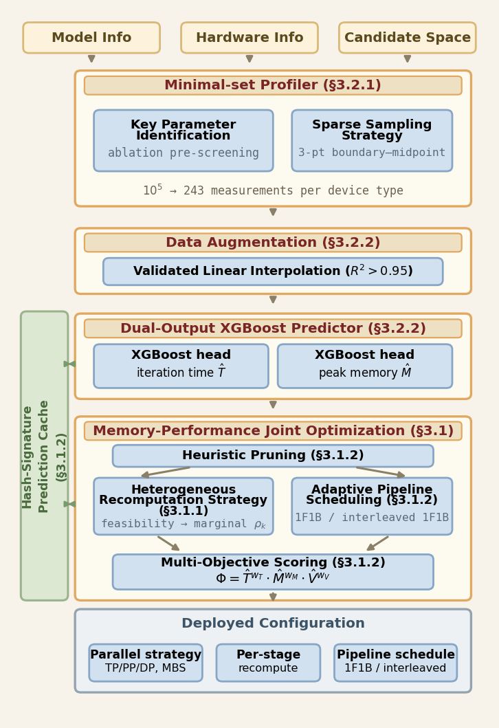
| Component | What it fixes | How |
|---|---|---|
| Per-stage recomputation | small-memory GPUs overflow while large-memory GPUs sit idle | each pipeline stage picks its own recomputation level (mostly Full or None) |
| Combined score Φ | a time-only search picks memory-imbalanced configurations | multiply time, peak memory and memory variance with weights |
| Few measurements + interpolation + XGBoost | too many configurations to measure each | measure three points per key parameter, interpolate, train a predictor |
| Prediction cache | even model calls get slow over tens of thousands of configurations | configurations with the same key parameters reuse the earlier prediction |
Per-stage recomputation: small-memory GPUs compute twice, large-memory GPUs do not
Existing systems usually switch activation recomputation on or off for the whole cluster. MemX lets each pipeline stage (usually one GPU type) choose its own recomputation level. Full saves the most memory: it keeps only each layer's input and reruns the whole layer's forward pass during backward. The deployment experiments have two full-layer options, full-block and full-uniform, and the paper does not say which of them the method's Full corresponds to. None keeps everything and recomputes nothing, so it costs no extra time. The middle level, Selective, keeps only some of the expensive intermediate results and recomputes the rest during backward; the paper found that it saves little memory on modern GPUs and its time cost cannot be told apart from measurement noise, so on such GPUs MemX drops this level and chooses only between None and Full (Section 3.1.1).
MemX decides each stage's level in two steps, and every candidate configuration goes through them during search. The first step makes sure it fits: if a stage does not fit even with Full, the configuration is pruned; if it fits with None, None is kept; otherwise Full is forced. The second step refines the choice among the levels that fit, aiming at the shortest total iteration time, based on each GPU type's marginal exchange rate (Eq. 1), that is, the extra time paid per MiB of memory saved. For this heterogeneous recomputation strategy, the paper does not explain how the recompute levels already listed in the candidate configurations connect with these two steps, nor give a concrete rule for changing a stage's level by the exchange rate. Configurations that pass both steps then get the combined score in the next section, and the lowest score wins.
The paper observes that the exchange rate depends on both compute and memory bandwidth: a compute-rich GPU with tight memory bandwidth can get bottlenecked by frequent recomputation, while a compute-poor GPU with ample bandwidth pays relatively less extra time for Full.
Applied to Table 1 as an illustration (the paper does not run MemX on this example): X, short of memory, could take a few more layers with Full while Y stays at None, which may bring the two stages' times closer; whether it does depends on how much time Full costs on X.
The combined score: any term that grows is penalized
Each candidate has three numbers: iteration time T, peak memory M (the highest of all GPUs), and memory variance V (how far each GPU's memory use in MiB is from the mean, counted in absolute usage, not as a share of capacity). Each is divided by a reference value (the paper's example is the median over feasible candidates), so it reads as "how many times the median", and then they are raised to their weights and multiplied:
The weights sum to 1 and read directly: if one term rises by 1%, Φ rises by roughly w percent. A weighted product makes each weight read as such an elasticity and lets any single term that is clearly too large pull the score up. A small constant is added to V so that a configuration with exactly zero variance does not drive the whole score to zero. A worked example (illustrative): configuration A takes 1.1 times the median time and has half the median variance; configuration B equals the median on both; both have median peak memory. With the default weights (0.4, 0.2, 0.4), A scores 1.1^0.4 × 0.5^0.4 ≈ 1.039 × 0.758 ≈ 0.79, and B scores 1. A is 10% slower but wins because its memory is much more even.
To avoid tuning weights on test data, all three weight profiles are chosen from the deployment conditions before evaluation, not picked after seeing results. The default profile (0.4, 0.2, 0.4) is for clusters with large differences between GPU types. A safety profile (0.3, 0.5, 0.2) is used when the cluster's minimum predicted memory margin falls below 10%, so avoiding OOM comes first. A throughput profile (0.7, 0.2, 0.1) is for homogeneous or weakly heterogeneous clusters (Section 3.1.2). In practice the paper also uses one profile per set of experiments: the ranking experiments on the 20-GPU cluster use the default profile, and the 6-GPU cluster, which has the tightest memory margin, uses the safety profile for the whole deployment experiment. The paper argues balanced memory brings three benefits: occasional memory spikes in a long training run are less likely to hit OOM; later increases in micro batch or sequence length leave room on every GPU; and the configuration is easier to move to a different set of GPUs. These three points are the paper's argument; the experiments do not test them separately.
How do tens of thousands of configurations become affordable to search?
For LLaMA2-7B on 16 GPUs, counting only the parallel layout, the layer split, per-stage recomputation and a few hyperparameters, the space already reaches about 10^8 configurations (Section 2.3). MemX's approach is measure little, estimate much, and reuse whenever possible.
Measure little: because most parameters barely change time or memory, it first runs single-parameter sweeps on each GPU type, changing one parameter at a time and watching how much iteration time and memory move. Only parameters that move them a lot (such as TP degree, recomputation level and micro batch size) are included in measurement; the rest are fixed at defaults. This cuts the dimensions to measure from more than ten to three to five. Each included parameter is measured at only its minimum, maximum and middle value, so the number of runs falls sharply: five parameters with ten values each would need 100,000 runs in full, while three points each need only 3^5 = 243.
Estimate much: first check whether interpolation is safe. On a representative device, a parameter interval is densely measured at five to seven points and fitted with a line; only if R² exceeds 0.95 is linear interpolation used inside that interval. Layer count against memory and micro batch against throughput are nearly straight lines. Sequence length against iteration time is superlinear (R² only 0.78, because attention cost grows with the square of length), so the interval is narrowed or not interpolated. The number of query groups barely affects throughput (a 0.8% difference), so it is fixed at the default (Figure 3d). After this the data typically grows five to ten times, and an XGBoost model is trained that gives iteration time and peak memory in one call.
Reuse whenever possible: the model predicts the time and memory of one pipeline stage processing one micro batch, trained on measured per-GPU time and peak memory. The full iteration time is then assembled with the 1F1B schedule formula: (number of micro batches − 1) × the slowest stage's time, plus the sum of stage times, the activation transfers back and forth between stages, a fixed overhead and data-parallel synchronization time; the synchronization time is estimated by formula from parameter size and bandwidth (Section 3.1.2). On the memory side, M is the largest predicted per-GPU peak and V is the variance of the per-GPU peaks; the paper does not explain how the per-micro-batch stage memory estimate is combined with the number of in-flight micro batches to get the end-to-end per-GPU peak for the whole iteration used in OOM pruning and Φ scoring. Each stage-level prediction gets a signature from its TP layout, recomputation level and other hyperparameters, and identical signatures take the cached result; the paper does not give the full signature fields, so a reader cannot judge whether a cached prediction still applies to a stage with a different number of layers. The cache is invalidated only when the GPU type, the model structure (such as layer count or hidden size) or the batch size changes. So when the cluster grows and only new PP and DP combinations appear, almost all new configurations hit the cache: 31,240 configurations (about 14 times the base space) take 26.5 seconds, only 6.5% more time than the base space. Adding micro-batch options invalidates the cache, and time grows linearly with the number of configurations (Section 4.3). Because it is unclear how cache entries are told apart when layer counts change, these numbers show only that the search is fast, not that the reused predictions stay accurate, and the paper gives no separate error for those reused predictions.
Experiments: is the prediction accurate, is the ranking right?
To create the condition where memory and compute are out of proportion, the main experiment uses a three-vendor, 20-GPU cluster: 4 A100s (80GB), 8 vendor-B GPUs and 8 vendor-C GPUs (both 32GB), with 28 GB/s between nodes. Built on Megatron-LM 0.8, it measured 36,740 training records over 1,628 distinct configurations, with models LLaMA2-7B/13B/70B and LLaMA3-8B/70B (Sections 4.1 and 4.2).
| Method | Configurations searched | Search time | Iteration-time MAPE | Spearman, time ranking | Spearman, Φ ranking |
|---|---|---|---|---|---|
| AMP | 14 | 40.07 s | 66.44% | 0.31 | 0.13 |
| Metis | 123 | 2.43 s | 14.91% | 0.87 | −0.07 |
| HexiScale | 24 | 0.253 s | 43.52% | 0.50 | 0.04 |
| FaSOP | same as AMP | same as AMP | 54.40% | 0.50 | 0.00 |
| MemX | 2,240 | 24.87 s | 12.17% | 0.90 | 0.93 |
(Tables 5 to 8. FaSOP is not open source; the authors re-implemented it on AMP's code, so its search cost equals AMP's.)
The table shows three things. First, MemX searches 160 times AMP's space in only 62% of AMP's time, because each configuration costs one millisecond-level model call, while AMP measures each one. Note this counts only the online search: MemX's time excludes offline profiling, interpolation and predictor training, while AMP's figure already includes its profiling. Second, its prediction error is the lowest; like Metis it has no configuration above 50% error, and its maximum error is 29.77%; FaSOP's MAPE rises to 76.47% on configurations with micro batch 2. Third, under the time ranking Metis is already close, but only MemX's first pick is the truly fastest configuration.
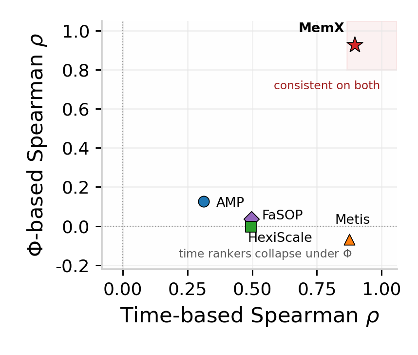
Under the Φ ranking all four baselines are close to random. Metis ranks time best (0.87) but drops to −0.07 on Φ. The paper explains that these methods do not optimize memory balance at all, so even an accurate time predictor cannot find balanced configurations. Note that this comparison is not quite fair to them: Φ is MemX's own objective, so this column mainly shows that "time alone cannot find balanced configurations", not that the baselines predict worse.
Real deployment: 9.3% slower, in exchange for the most even memory
Everything above is prediction and ranking. To see how recommended configurations actually run, the paper trains a 6-layer LLaMA-2-style model on a 6-GPU cluster (4 V100s plus 2 T4s), measures 226 configurations, and uses the safety profile for Φ (Section 4.4, Table 10).
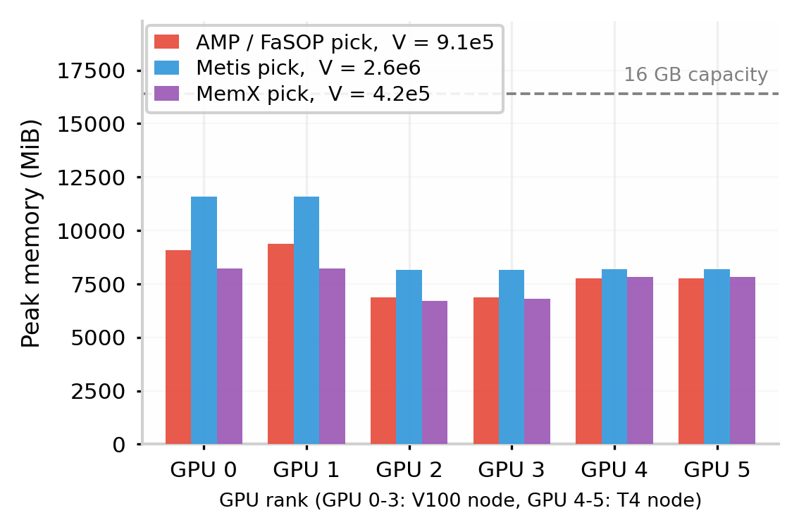
On time alone, AMP, FaSOP and MemX all find the truly fastest configuration (9,211 ms), so the baselines do not fall behind. Metis recommends a micro-batch-4 configuration that ranks only 28th to 60th; HexiScale does not search recomputation, and its recommended configuration runs out of memory without it. The MemX configuration chosen by Φ has exactly the same parallel skeleton as AMP's: tensor parallelism of 2, a 3-stage pipeline, no data parallelism, micro batch 2. The difference is that it turns on full-layer recomputation and uses sequence length 1024, 64 attention heads and 16 query groups, none of which the baselines search. Note that sequence length and head count also change the training job itself, so the time and memory differences below cannot all be credited to recomputation; the paper does not separate them.
It takes 10,066 ms, 9.3% slower than the fastest configuration, which shows it deliberately spends time to buy memory: its memory variance is only 4.19×10^5, ranking first on Φ among all 226 configurations, while the fastest configuration has variance 9.13×10^5 and ranks only 20th on Φ. The cost of recomputation itself is in the 18 matched groups of Figure 8. In this experiment the recomputation strategy has four values, none, selective, full-block and full-uniform, which go into the configuration space like any other parameter, with the predictor estimating their time and memory. full-block and full-uniform are two kinds of full-layer recomputation, named after the Megatron-LM options of the same names, and full-uniform saves more and costs more time. The paper does not say which layers full-block recomputes, so the Full in the two-step assignment cannot be equated with these deployment options. full-block, which MemX deployed, saves 7.6% of peak memory at a median 8.5% extra time; full-uniform saves 13.9% for 19.2%.
In this example the two goals really conflict: across the 226 configurations, the correlation between time rank and Φ rank is only 0.66.
The paper also extends the 20-GPU measurements along the pipeline to simulate 40 and 60 GPUs: iteration-time MAPE rises from 12.17% to 14.22% and 16.19%, memory MAPE stays around 6.5%, and Spearman falls from 0.90 to 0.87 (Table 11). The "ground truth" in these simulations is itself derived from the 20-GPU data by compute ratios, and the paper admits it only shows the prediction pipeline is self-consistent and cannot replace real large-cluster validation.
Where I think it falls short
First, it does not show faster training. MemX's selling point is what balanced memory brings: fewer OOMs, room to change hyperparameters, easier migration to other GPUs. But in the only real deployment its pick is 9.3% slower than the fastest configuration, and none of those three benefits is tested on its own, for example by counting OOMs over a long run.
Second, the evidence for "the only method that finds the real best configuration" is thin. Top-1 is a single hit under each ranking. Deployment validation covers only one 6-GPU cluster with a 6-layer model; on the 20-GPU cluster only prediction and ranking are compared, and the configurations recommended by each method are never actually trained to compare throughput. Also, the core idea, more recomputation on small-memory GPUs and none on large ones, is never tested on its own: no recommended configuration mixes recompute levels across stages, and there is no ablation without it; MemX's pick on the small cluster turns on full-block recomputation for the whole configuration.
Third, the conclusions depend on weights chosen in advance. The three profiles emphasize different things and may pick different configurations, but the paper does not test how the recommendation changes with the weights. Larger scale is only simulated from 20-GPU data, only by extending the pipeline, so changes in cross-node communication are not captured. Also, the text gives 14.91% as the 60-GPU MAPE while Table 11 and Figure 10 give 16.19%; since the two disagree, this article follows Table 11.
How a search or recommendation team could try it
Teams training large models or ranking models on GPUs of different models or vendors can try it in steps:
- Measure the current state: under the current configuration, record each GPU's peak memory and compute the variance across GPUs and the smallest margin. If margins are ample and variance is small, there is no need to change anything.
- Try the score at zero cost: re-rank configurations you have already measured by Φ with the default weights, and check whether the top one differs from the fastest, how much slower it is, and how much lower its variance is.
- Try per-stage recomputation: turn on full-layer recomputation only on the pipeline stage with the tightest memory and leave the other stages off; measure how much iteration time rises and how much peak memory and variance fall, and compare with the paper's full-block figure of 8.5% time for 7.6% memory.
- Add a predictor only when the configuration space is large: run single-parameter sweeps first to find the parameters that matter, measure three points for each, check R² before interpolating, then train a model that predicts time and memory together, and track its prediction error.
Conclusion and assessment
The main takeaway: on a cluster where memory and compute are out of proportion, a parallel-configuration search should put both memory level and memory balance into its objective and let different GPUs use different recomputation levels; minimizing time alone can pick a configuration that runs some GPU right at its memory limit.
| Dimension | Assessment |
|---|---|
| Importance of the problem | Medium-high. Mixed-vendor clusters are increasingly common, and the split between memory and compute is a real problem |
| Novelty of the method | Medium. Per-stage recomputation and memory balance as an objective are new; measurement plus interpolation plus XGBoost plus caching combines known ideas |
| Experimental evidence | Medium to weak. Prediction and ranking data are large, but real deployment is one 6-GPU cluster and larger scale is only simulated |
| Engineering cost | Medium. It needs configuration search on Megatron-LM and a few measurements per GPU type; the code is open source |
| Worth trying? | Steps 2 and 3 are worth doing first; the payoff is largest on mixed clusters that often hit OOM or memory imbalance |
How did this read for you?
Hoot made a note. Thanks for the feedback.

One tap, no sign-in; tap again to undo. Only anonymous counts are kept, never who you are.
Discussion
Add experiment details, reproduction notes or a different take. Requires a GitHub sign-in.
Loading the discussion…