Contents · 8 sections
1What problem is it actually solving?2The overall structure: two libraries in layers3Why doesn't splitting into modules slow things down?4The two-stage index: find coarsely, then rank precisely5Results6Where I think it falls short7How a retrieval team could try it8VerdictSHARE

In vector search, switching to another embedding form or quantizer often means switching libraries. Existing ANN libraries either support one combination or write separate code for each, and no ANN library covers dense, sparse and multi-vector embeddings behind one interface. The authors release two open-source Rust libraries to fix this: Vectorium stores vectors, computes distances and quantizes, and kANNolo builds HNSW and IVF indexes on top of it. Every combination is compiled into specialized code, so splitting things into modules costs no run-time speed. Their two-stage HNSW first finds candidates on compressed vectors, then rescores them with more precise vectors. On dense data at 99% recall, it handles 2.5 to 3.3 times as many queries per second as the reference HNSW implementation, with an index half the size. Teams running both dense and sparse retrieval should read it, because it shows modularity and speed can coexist when the cost is paid at compile time.
What problem is it actually solving?
Start with an illustrative scenario. A question-answering search team has two retrieval channels: one uses 768-dimensional dense embeddings, the other uses learned sparse vectors such as SPLADE. The team now wants to do three things.
| What the team wants (illustrative) | Usual approach |
|---|---|
| Replace PQ with RaBitQ in dense retrieval | Switch to a library that implements RaBitQ and rewrite the build and query code |
| Use a graph index for sparse retrieval too | Find another graph library that supports sparse vectors |
| Rescore sparse candidates with a multi-vector model | Write glue code that matches the two libraries' results by id |
The trouble is that vector form, index structure, distance and compression are largely independent choices, yet existing libraries tie them together. Faiss, the most widely used dense-vector library, writes one class for each combination of index structure and quantizer, and each class has its own build and search code. More combinations mean more code, and adding a new quantizer touches many places. Newer modular libraries split only one side: ParlayANN and ANNLib split the graph-index side, and Glass splits the quantizer side.
The paper's contribution is to pull all four choices apart: the index goes to kANNolo, and the other three go to Vectorium. Swapping the quantizer changes one type parameter and not a line of index code. The split also costs no speed, for the compile-time reason explained below.
The overall structure: two libraries in layers
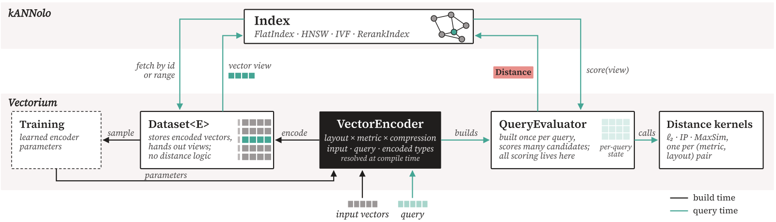
The lower layer, Vectorium, manages data. It divides the path from storing a vector to scoring it into four parts, each stacked on the previous one:
| Part | What it handles |
|---|---|
| Vector view | How one vector is laid out in memory (dense, sparse, packed codes, multi-vector), read without copying |
| Distance | A score, plus whether larger or smaller is better |
| Encoder (VectorEncoder) and query scorer (QueryEvaluator) | The encoder compresses raw vectors into a stored format; the scorer scores a query against that format |
| Dataset | Stores a batch of encoded vectors and hands them out by id |
Vectorium has 11 encoders, from uncompressed 32-bit floats down to codes using less than one bit per dimension. Its PQ matches Faiss in accuracy, and its RaBitQ scan is 1.4 to 2.4 times faster than the original authors' implementation.
The upper layer, kANNolo, manages indexes. It implements HNSW and IVF, each generic over vector form, encoder and distance. It also has a two-stage index, RerankIndex, covered separately below.
The key to this split is that storage and scoring are separate. A Dataset holds no distance logic, and all scoring goes through the scorer that comes with the encoder. So the same HNSW search loop can run on f16 dense vectors, on PQ codes or on sparse vectors.
Why doesn't splitting into modules slow things down?
Modules usually have a cost. The common approach calls the distance function through a shared interface inside the search loop, which adds one indirect jump per call. One HNSW query computes many distances, so this overhead adds up.
Vectorium makes encoders and datasets generic parameters, and lets the Rust compiler generate a separate copy of the code for each combination. This is called monomorphization. As an analogy, a shared interface is like a universal remote that must check which TV it is connected to before every button press. Monomorphization gives each TV its own dedicated remote, so each press works directly.
In each specialized copy, the distance computation is inlined into the search loop, with no indirect call left. The authors measured the alternative: calling the distance function dynamically through a Rust trait object makes each distance computation take 1.07 to 1.52 times as long when the data sits in cache. Under random memory access, which is what graph search mostly looks like, it is at most 7% slower.
The cost moves to compile time. kANNolo's Python bindings precompile every combination they expose. A full release compile takes 113 seconds and produces a 5.3 MiB library. The beam search alone is compiled 164 times, once per combination of graph layout, encoder and distance, and these copies make up 3.1% of the generated code.
Run-time speed is bought with compile time and library size. For someone calling the libraries directly from Rust, the price is small, because a program compiles only the combinations it uses. For Python users, a combination missing from the bindings needs a new binding class and a recompile.
The two-stage index: find coarsely, then rank precisely
The two-stage index, RerankIndex, first appeared in the authors' earlier work on sparse retrieval with multi-vector rescoring. This paper makes it a general component: any index can be the first stage and any dataset the second, joined into one index. The first stage finds candidates with a cheap representation, and the second stage rescores them with a more accurate one.
The two stages can use different encodings and distances; the only requirement is that their vector ids line up. The paper gives several ways to combine them:
- the first stage searches a graph over PQ-compressed vectors, and the second holds a high-precision copy of the same vectors;
- the first stage finds candidates with HNSW over sparse vectors, and the second rescores them with multi-vector embeddings and MaxSim. Here the query is also encoded in both forms, sparse and multi-vector, and each form goes to its own stage;
- the two stages each store one part of the same vector. For example, the largest entries of a sparse vector go into the first stage and the rest into the second. The query stays whole, and each stage computes its inner product with its own part. The first-stage score is used to find candidates; the second stage then scores the remaining part of each candidate and adds the first-stage score, which gives the exact inner product. The final ranking uses this sum.
A query takes two steps: the first stage retrieves candidates, and the second stage scores each candidate with the full representation and keeps the top . Two optional pruning steps make the second stage do less work.
The first is candidate pruning. Here the first-stage scores are read as similarities, so higher is better. Let be the first-stage score of the candidate in position . Candidates scoring below are dropped. An illustrative example: with , a 10th-place score of 0.80 and , candidates below 0.72 never reach the second stage. This threshold form assumes positive scores. The step also relies on the two stages' scores broadly agreeing.
The second is early exit. The first-stage candidates are already sorted by score, and the second stage rescores them in that order. If candidates in a row fail to enter the current top , it stops and skips the rest.
The third combination is used for sparse vectors, and it is how the sparse kANNolo-Rerank in the experiments is configured. kANNolo splits each sparse vector into two parts: the entries with the largest absolute values go into the first part until their absolute values add up to of the sum of all entries' absolute values, and the rest go into a residual. The graph is built only on the first part, and the residual is used for rescoring. Hoot says

- The split: 0.5 plus 0.3 is 0.8, exactly 80% of the whole vector, so these two go into the first part.
- The scores: let the query be 2, 1, 1, 3 at these 4 positions (illustrative). The first part scores 1.3, the residual 0.4, and together 1.7, the same as the inner product with the whole vector.
All numbers are illustrative. The large entries go into the first part, and the graph is built only on that part, so the graph is smaller and faster to search. The residual plays no part in finding candidates and is used only at rescoring. Adding the two scores drops no entry. Source: paper §5.1 RerankIndex residual mode and §6.1 sparse kANNolo-Rerank setup
Here is an illustrative calculation. A sparse vector has 4 nonzero entries, 0.5, 0.3, 0.1 and 0.1, and . The first two add up to 0.8, exactly 80%, so the first part is 0.5 and 0.3 and the residual is the two 0.1 entries. The query's inner product with the vector equals its inner product with the first part plus its inner product with the residual. Adding the two scores gives the inner product with the whole vector, so splitting the vector drops no entry at rescoring time. Recall can still be lost, because the graph search and the two pruning steps above can each miss a true neighbor.
Results
The authors compare against 11 systems on 7 public collections, both dense and sparse. None of these collections was used in the earlier design studies, so the results were not measured on the data used for tuning. The main measure is Accuracy@10, called recall below: for each query, take the fraction of the index's top 10 that is also in the exact search's top 10, then average over all queries as a percentage. The comparison is how many queries per second each system handles at 90%, 95% and 99% recall.
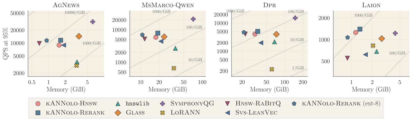
First, dense data against hnswlib. hnswlib is the reference HNSW implementation and stores uncompressed f32 vectors. kANNolo-Hnsw is the same kind of graph index but stores f16 vectors. kANNolo-Rerank is two-stage. Its graph is first built over the f16 vectors, and then the vectors in the graph are replaced by 1-bit RaBitQ codes, so the codes play no part in building it. RaBitQ is an existing quantization method that keeps 1 bit per dimension, so these codes only give rough distance estimates. The first stage uses these rough scores to find 100 candidates on the graph. The second stage rescores these 100 candidates on the f16 copy and keeps the top 10.
| Collection (99% recall) | kANNolo-Hnsw throughput vs hnswlib | kANNolo-Rerank throughput vs hnswlib |
|---|---|---|
| AgNews | 2.84x | 3.04x |
| MsMarco-Qwen | 2.70x | 3.26x |
| Dpr | 2.17x | 2.47x |
On these three collections, both kANNolo indexes are also about half the size of hnswlib's. This shows the throughput gain is not bought with extra memory. On Laion, whose queries come from a different distribution than the collection, hnswlib tops out at 98.74%, and only kANNolo and LoRANN reach 99%.
Collection size also decides who leads. On the small collections below 1.1 million points, kANNolo is not always first. For example, at 99% recall on AgNews, Glass handles 6,085 queries per second against 4,585 for kANNolo-Rerank. But Glass uses 2.0 times the memory of kANNolo-Rerank, so it is trading memory for speed.
On the two large collections of 8.8 million and 21 million points, kANNolo-Rerank is the fastest at every recall target apart from SymphonyQG, 1.15 to 1.39 times ahead of the next system. SymphonyQG is faster still, 1.81 to 3.36 times kANNolo-Rerank on Dpr, but it also uses about 4 times the memory. So in throughput per GiB of memory, kANNolo still leads.
How much is the two-stage design itself worth? Compared with kANNolo-Hnsw, which searches the graph directly over f16 vectors, the two-stage index has 1.07 to 1.20 times the throughput at 99% recall, and more at 90% and 95%, up to 41%. This shows that searching the graph over compressed codes and then ranking precisely in f16 is cheaper than searching the graph directly over f16 vectors.
On sparse data, the fastest systems are the inverted indexes Seismic and SeismicWave. They come from the same group of authors, are also built on Vectorium, and beat kANNolo-Rerank on every collection at every target. kANNolo-Rerank is the fastest graph index measured: 5.2 to 48.4 times faster than PyANN, the other sparse graph index, with a third of its memory. kANNolo's indexes also use the least memory on all three sparse collections.
Where I think it falls short
First, index building is not fast. For the 99%-recall configurations on Dpr, kANNolo's two indexes take 4,814 and 4,891 seconds to build. That beats hnswlib's 5,238 seconds, but Svs-LeanVec needs only 2,982 seconds. Svs-LeanVec is fast because it first reduces the vectors to 384 dimensions and one byte per dimension, then builds its graph. The authors note that among the eight systems, their build time most often ranks fourth or fifth.
Second, tail latency gets worse. The cause is when a search stops. Standard HNSW keeps a fixed-length candidate list and stops when the next point to expand is farther than the worst one on the list. kANNolo-Hnsw relaxes this line by a ratio λ: it keeps searching as long as the next point is no farther than the worst on the list by more than that ratio. This allows a very short candidate list, but the number of steps varies more from query to query. As a result the median latency drops while slow queries get slower. On AgNews at 95% recall, the median latency drops from 141 to 100 microseconds, while P99 rises from 226 to 308 microseconds. This shows that while the average gets faster, the slowest queries get slower.
The gap is wider at 99% recall. the P99 latency of kANNolo-Hnsw is 4.2 to 5.4 times its median, against 1.7 to 2.0 times for hnswlib. So looking only at median latency overstates the user experience. In absolute terms kANNolo's P99 is still below hnswlib's, and the two-stage index brings the ratio back down to 1.5 to 2.4.
Third, for sparse data a graph index is not the best choice. On MsMarco-E-Splade, Seismic is 4.13 to 17.6 times faster than kANNolo-Rerank. A team doing only sparse retrieval is better served by an inverted index.
How a retrieval team could try it
- Start with a baseline on existing dense retrieval. Store f16 vectors in kANNolo-Hnsw and compare throughput and memory with the production hnswlib or Faiss at the same recall. Go further only if neither is worse than production.
- Then try the two-stage index. Following the paper, build the graph over f16 vectors, replace the vectors in the graph with RaBitQ codes to find candidates, and rescore on the f16 copy. The best code width differs by collection, so sweep it yourself. Focus on the 90% to 95% recall range, where the paper shows the largest two-stage gain.
- To save memory, switch the second stage from f16 to 8-bit RaBitQ-ext. At 90% recall, throughput stays at 95% to 99% of the original and memory falls to just under 60%, which means the saving is nearly free at that level. At 99% recall, throughput drops by 25% to 38%, and on Laion, whose queries come from a different distribution, it cannot reach 99%. So check which recall level production needs.
- Teams with sparse retrieval can try the chain of a sparse graph for candidates plus multi-vector MaxSim rescoring, with both stages in one index and no glue code. This chain was measured in the authors' earlier work and is not re-measured in this paper.
Verdict
The most useful lesson of this paper: vector form, distance, quantization and index can be split into largely independent parts, and as long as each combination is compiled into specialized code, the split costs no speed.
| Dimension | Assessment |
|---|---|
| Problem importance | High. Multiple embedding forms in one system are now common, and the cost of switching libraries is a real engineering burden |
| Method novelty | Medium. Monomorphization is standard Rust practice; the contribution is splitting the whole design space systematically and making the two-stage index a general component |
| Experimental evidence | Strong. 7 collections, 11 competing systems, and the main claims are backed by ablations |
| Engineering cost | Medium. Low for Rust users; Python users are limited to the combinations precompiled in the bindings |
| Worth trying? | Yes, especially for teams running both dense and sparse retrieval who want to compare quantizers quickly |
How did this read for you?
Hoot made a note. Thanks for the feedback.

One tap, no sign-in; tap again to undo. Only anonymous counts are kept, never who you are.
Discussion
Add experiment details, reproduction notes or a different take. Requires a GitHub sign-in.
Loading the discussion…