Contents · 9 sections
1What problem is it actually solving?2Overview: the steps from training to serving3Why train the MTP head again after post-training?4How does 4-bit quantization keep accuracy?5Serving: where does the throughput come from?6Main results7Where I think it falls short8How a recommendation or search team could try it9Is it worth reading?SHARE

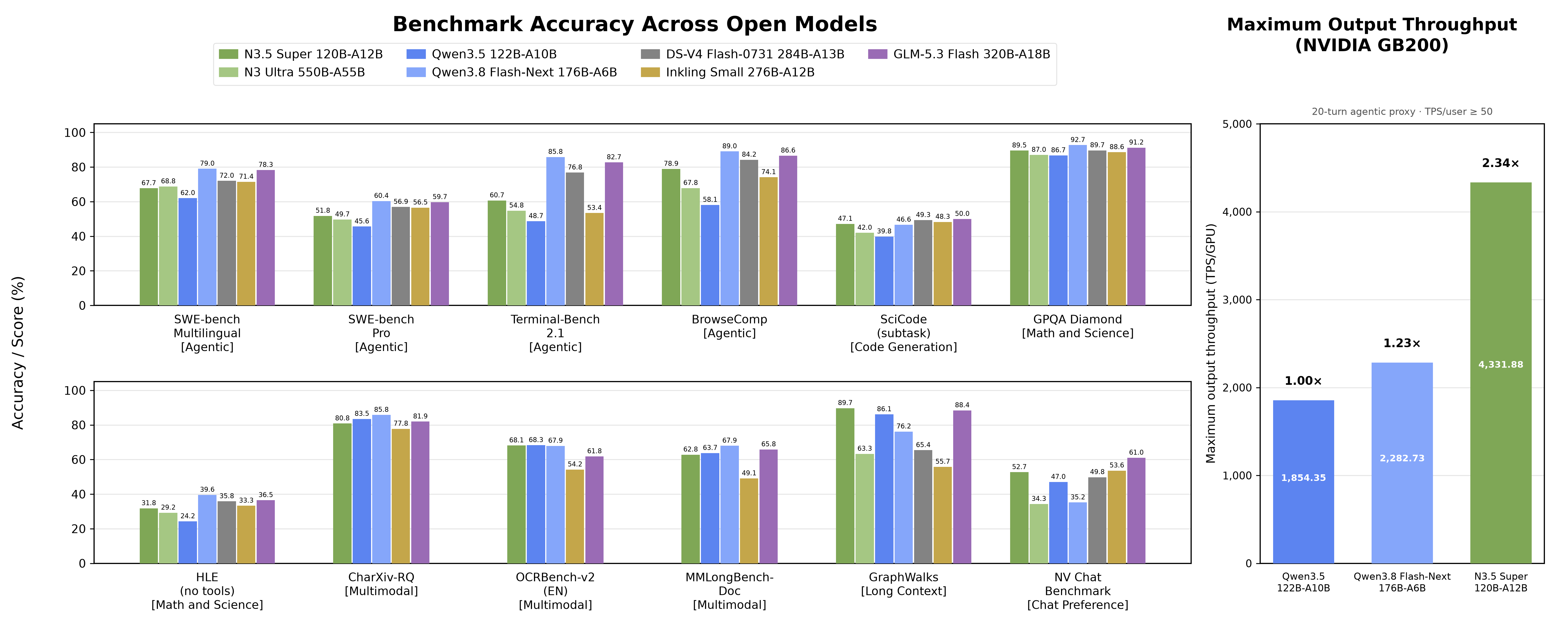
Open models built for agents often have to choose between capability and inference cost. NVIDIA's Nemotron 3.5 Super optimizes both. It is a hybrid Mamba-Transformer mixture-of-experts model that activates only about a tenth of its parameters per token, and it scores 51.78% on SWE-bench Pro, ahead of the previous-generation Ultra with several times more active parameters. The deployment design matters more to people who serve models. The model carries its own multi-token prediction head for speculative decoding, and post-training trains that head again, raising the average number of accepted tokens per step over the original head by 21.8% when drafts are sampled and by 10.1% under greedy decoding. With NVFP4 quantization, throughput on an interactive agent workload is 2.43 times that of BF16. Base, post-trained and quantized weights are released together with the training data.
The technical report is long and covers pretraining, Indian-language data, multimodality and reinforcement learning. For teams that serve models, three parts are worth reading closely, because they can be copied directly. First, the draft head needs its own re-alignment after the backbone is finished. Second, 4-bit quantization gives different modules different precisions and then recovers accuracy with a few hundred steps of distillation. Third, the Mamba state is written to GPU memory far less often during speculative decoding. This piece covers only those three and touches model capability briefly.
What problem is it actually solving?
First, how this paper uses its multi-token prediction head (MTP head). Nemotron has a single MTP head attached after the backbone's last layer and calls it repeatedly: each call guesses one more token, so seven calls give seven draft tokens. The backbone then checks all of these guesses in a single forward pass: the leading correct guesses are kept, and everything from the first wrong guess onward is thrown away. The average number of tokens kept per step is the acceptance length (AL). The higher the AL, the fewer backbone forward passes are needed for the same number of tokens.
The trouble is a misalignment, in two senses. The first is a version mismatch. After SFT, the backbone still goes through reinforcement learning and multi-teacher distillation, and its output distribution keeps moving. The MTP head is trained along with it in these stages, but their goal is backbone capability, and the draft head does not keep up with the backbone's changes. Table 8 of the paper shows it: the SFT-stage model with its own MTP head reaches an AL of 4.589, while the final post-trained model with its own MTP head drops to 4.287 (greedy decoding). The backbone got better, and the draft head got worse at guessing it.
The second is a train–inference input mismatch. The MTP head is used recursively: for the 1st token it reads the backbone's hidden state, for the 2nd it reads the hidden state from its own first step, and so on. This shared recursive formulation comes from the Super 3 report, but Super 3 itself had two non-shared heads and 3.5 keeps only the first; the paper does not say exactly how, in each round, the previous round's hidden state, the draft token just guessed and the verified prefix are combined into the next round's MTP input. In ordinary training, step k reads the hidden states that step k−1 computed over the whole real text, all from the same source. Inference is different: tokens already verified have hidden states computed by the backbone, while the draft tokens just guessed in this round have hidden states computed by the draft head itself. So the context the draft head reads is stitched from two sources, and the further along the draft, the larger the self-computed part. The later the draft position, the further its input is from what it saw in training, and the faster acceptance drops.
An illustrative scenario. One reply from a coding agent has 1,000 output tokens, and the draft length is 7 (seven guesses per step):
| Illustrative | Tokens kept per step | Backbone forward passes for 1,000 tokens |
|---|---|---|
| No speculative decoding | 1 | 1,000 |
| Original MTP head after post-training, sampled decoding | 3.787 | about 264 |
| Re-aligned MTP head, sampled decoding | 4.612 | about 217 |
The AL values come from Table 8 of the paper (temperature 1, drafts sampled by probability); the pass counts are illustrative estimates, 1,000 divided by AL. Forty-odd fewer forward passes per reply adds up to real latency over a 20-turn agent session.
Overview: the steps from training to serving
The deployment-related steps, in order:
| Stage | What happens | Output |
|---|---|---|
| MTP initialization and warm-up | Keep only the first of Super 3's two MTP heads and turn it into one reused head; freeze the backbone and train only this head for 100 billion tokens | A draft head that guesses several tokens recursively |
| Distillation and mid-training | Distill 1 trillion tokens from the larger Ultra 3, then add long-context and software-engineering data | Base model |
| Post-training | SFT, RLVR, RLHF, multi-teacher distillation | Final backbone (now misaligned with the MTP head) |
| MTP re-alignment (the paper calls it MTP boosting) | Freeze the backbone and update only the MTP head | A draft head aligned with the final backbone |
| Quantization | Use NVFP4 and FP8 for different modules, quantize directly, then run 200 steps of distillation to recover accuracy | Released weights at 4.82 bits per parameter |
| Serving | Prefix reuse in vLLM, fine-grained kernel choice, a replay scheme for the Mamba state | Production configuration |
The division of labour: MTP re-alignment decides how many tokens each step keeps, and quantization decides how long each step spends reading weights, while the serving changes let more requests run at once. The parts one by one follow.
Why train the MTP head again after post-training?
If post-training misaligns the draft head, the direct fix is to align it once more after post-training ends. The paper's recipe has three key points.
First, the backbone is fully frozen and only the MTP head is updated. This step cannot change model capability, so benchmarks need no rerun, and the risk is small.
Second, the training data is the final backbone's own replies. The authors take prompts from public post-training datasets, let the backbone sample at temperature 1, generate replies up to 8K tokens, and compute the loss only on the reply tokens. The draft head has to guess what the backbone will actually say in production, so the backbone's own output is the right training material.
Third, the supervision changes from "guess the next real token" to "match the backbone's whole probability distribution", that is, distillation with the frozen backbone as teacher. For MTP boosting, the paper does not say whether, from the second recursive step on, the teacher distribution is computed by the backbone on the real prefix of the reply or on the prefix the draft head guessed recursively. Why change the supervision? Under sampled speculative decoding, the method is rejection sampling: for each draft token, the probabilities the backbone and the draft head give it are compared to decide whether to keep it, and a rejected position is filled by sampling a new token. A draft head that has only learned "the single most likely word" has a differently shaped distribution and gets rejected more often under sampling. The paper says this supervision especially helps non-greedy sampling, and Table 8 agrees: the gain at temperature 1 (3.787 to 4.612) is much larger than under greedy decoding (4.287 to 4.718).
For the second mismatch, the authors keep a training trick called hidden-state mixing. In plain recursive training, all of step k's input comes from step k−1's output. The paper describes this trick in a single sentence: at training step k, the input hidden states are sampled from the states produced by steps 1 through k−1, rather than always from step k−1. For hidden-state mixing, the paper does not say whether this sampling is done token position by position or for a whole sequence at once, nor whether the backbone's hidden states are among the candidates. The purpose is clear: let the draft head read hidden states of mixed origin during training, closer to the stitched context it reads at inference. It is much cheaper than training methods that simulate the full inference process step by step (test-time training).
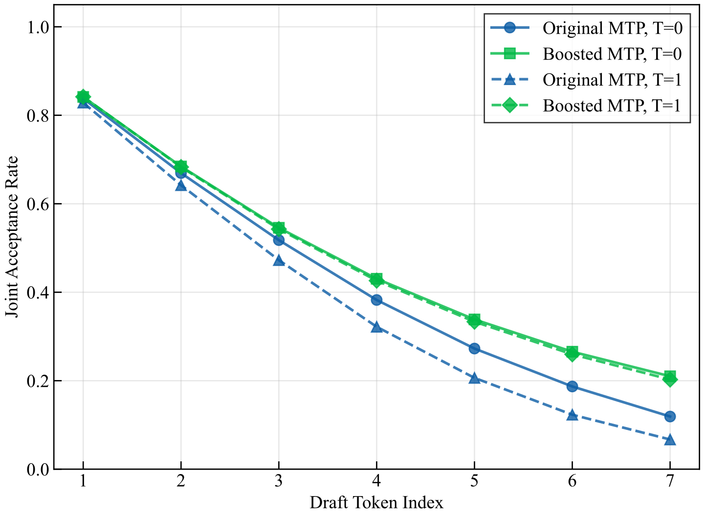
Figure 6 shows that the gain sits mostly in the later draft positions, exactly where the second mismatch is worst. The first position still reads the backbone's true hidden state and is nearly unchanged.
One more cost-saving detail. The authors first trained the MTP head for 4,000 steps on the SFT-stage backbone, and this run converged quickly. Moving that head straight onto the final backbone already brings AL from 3.787 back to 4.436 (temperature 1); another 25,000 steps on the final backbone reach 4.612. In other words, most of the gain from a head trained early carries over to the later backbone, so after post-training only a shorter top-up run is needed.
| MTP head state (SPEED-Bench, draft length 7) | Greedy AL | Temperature-1 AL |
|---|---|---|
| SFT backbone + its own head | 4.589 | 4.048 |
| SFT backbone + 4,000 steps | 5.080 | 4.730 |
| Final backbone + its own head | 4.287 | 3.787 |
| Final backbone + head moved over from the SFT-stage run | 4.528 | 4.436 |
| Final backbone + 25,000 more steps | 4.718 | 4.612 |
How does 4-bit quantization keep accuracy?
Compressing a 120B model to NVFP4 is hard mainly because different parts tolerate quantization very differently. The authors used NVIDIA's AutoQuant tool to estimate a sensitivity per module: quantizing a module pushes its output away from the original, and that deviation is weighted by the squared gradient of the task loss with respect to the output, so a large deviation in a loss-sensitive place scores high. The result is very uneven: the output layer (lm_head) alone accounts for nearly half of the total NVFP4 sensitivity, attention and Mamba projections come next, and the MoE experts are the most robust.
This is the reverse of how parameters are spread: experts hold most of the parameters yet fear quantization least. The release does not use a recipe produced by the sensitivity search. It uses a predefined aggressive recipe whose tiers agree with this sensitivity profile: it puts the matrix multiplies of the MoE experts and shared experts in NVFP4, uses FP8 for attention projections and Mamba linear layers, and keeps the output layer at a precision higher than NVFP4. Counting quantization scales, the whole model averages 4.82 bits per parameter, about 75 GB of weights.
"How much of the score is kept" uses one definition throughout: for each benchmark, divide the quantized model's score by the BF16 score, then take the median of these ratios across benchmarks. Quantization loses some accuracy, and QAD (quantization-aware distillation) closes the rest by training the quantized model for a few hundred more steps: only the quantized matrix-multiply weights in the language model are updated, all other parameters stay frozen, and on the post-training SFT blend a KL divergence objective pulls the quantized model's output distribution toward the model before quantization. The authors found that the best step count depends on the recipe: for the released 4.82-bit recipe, 200 steps was best and 300 was slightly worse, so the release uses 200. On 36 benchmarks, this median is 99.62% for the released quantized model, and replies are only 0.44% longer on average. Reply length is the second metric the authors watch on purpose: if a quantized model gets wordier, the extra tokens eat the compute it saved, so the acceptance criteria cap the length increase at 5%.
Serving: where does the throughput come from?
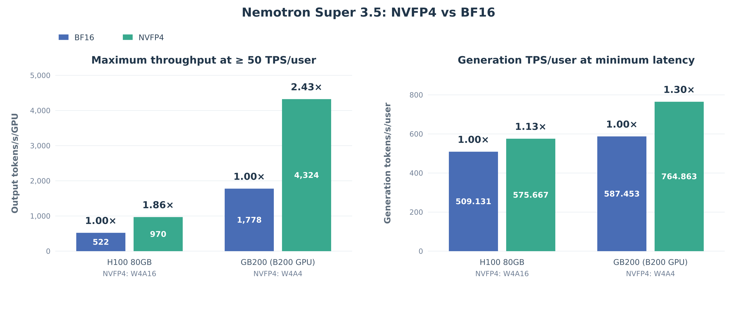
The test workload resembles a real agent session: a shared prefix of about 50K tokens, then 20 turns with 2K input and 1K output each. Only configurations giving each user at least 50 output tokens per second count; slower points do not count even if their total throughput is high.
The authors attribute the throughput lead to three things. First, the model has only a few attention layers and uses Mamba-2 for the rest. The Mamba state has a fixed size that does not grow with context, so as an agent session gets longer, each request's memory grows slowly, more requests fit on one GPU, and they share the cost of each weight read. Second, the MTP head's high AL means each forward pass keeps more tokens. Third, the model's LatentMoE design sends each token to its experts as a compressed vector smaller than the hidden state, so under multi-GPU expert parallelism each token moves less data across GPUs.
Mamba also brings a problem specific to speculative decoding. For each incoming token, a Mamba layer updates its fixed-size state: new state = decay factor × old state + the outer product of that token's key and value. Speculative decoding verifies 7 draft tokens at once without knowing how many will be kept, so it has to write every possible new state back to GPU memory. Longer drafts mean more writes; this step is purely memory-bandwidth bound and also limits how many requests can run together.
The authors' fix is "checkpoint plus replay" (developed concurrently and independently of the Dao lab's ReplaySSM). GPU memory holds a single state from one moment (the checkpoint), and afterwards each token only records its small key, value and decay factor in a buffer. When a batch of drafts is verified, each position's output does not need the state written out first: the output is the sum of two parts. One part is the query times the checkpoint state, multiplied by the product of the decay factors of every step since the checkpoint. The other comes from each buffered record: the dot product of the query with that record's key gives a weight, which multiplies the record's value and then the product of the decay factors of the steps after that record. This gives the same result as first computing the state with the recurrence and then multiplying by the query, and the full state can be rebuilt on the spot from the checkpoint and the records when it is needed. After verification the buffer keeps only the accepted tokens, a rejected draft just moves a counter back, and the next batch of drafts appends to the same buffer. Only when the buffer is full (16 steps in the paper's experiments) is the state actually computed and written back to GPU memory once, as the new checkpoint. As a result, where each verification used to write T possible new states back to GPU memory (T is the draft length), the state is now written back only once the buffer has filled with a number of tokens. State-related memory traffic drops sharply, and the memory saved lets more requests and longer drafts run at once. On a single GB200, turning it on raises total throughput by 4.7% to 6.4% and per-user speed by 6.4% to 12.5%.
Main results
| Item | Compared with | Result |
|---|---|---|
| SWE-bench Pro | Nemotron 3 Ultra, about 4.6 times more active parameters | 51.78%, ahead of Ultra |
| Average MTP AL (temperature 1) | Original head after post-training, 3.787 | 4.612 after re-alignment, 21.8% more |
| Average MTP AL (greedy) | Original head after post-training, 4.287 | 4.718 after re-alignment, 10.1% more |
| Accuracy kept after quantization | BF16, 36 benchmarks | Median 99.62%, replies 0.44% longer |
| Throughput (GB200, at least 50 tokens per second per user) | BF16, 1,778 tokens/s per GPU | NVFP4, 4,324 tokens/s per GPU, 2.43 times |
| Throughput (same workload) | Qwen3.5 122B-A10B | 2.34 times |
Taken together, the speed lead does not come from one trick: architecture, draft head, quantization and serving each contribute a share. MTP re-alignment and QAD are the cheapest pieces, since both freeze most parameters and train only hundreds to tens of thousands of steps.
Where I think it falls short
First, the draft head's lead holds only under sampled decoding. In Table 9 of the paper, under greedy decoding Gemma-4 31B averages an AL of 4.837 and Qwen3.5 122B-A10B 4.799, both higher than the re-aligned Nemotron's 4.718; only at temperature 1 does Nemotron lead, 4.612 against Gemma's 4.565 and Qwen3.5's 4.331. This means that with greedy decoding in production, re-alignment still helps, but the lead over these two models disappears.
Second, the 2.43 times is available only on Blackwell GPUs. It relies on W4A4, while H100 can only run W4A16, where the same comparison gives 1.86 times, so teams running mostly Hopper GPUs will not get this large a gain. The released checkpoint also uses an FP8 KV cache; the KV cache is not compressed to 4 bits.
Third, the quantization search is not cheap. Each candidate recipe needs about 1,024 GB200 GPU-hours per 100 QAD steps, and the authors compared three recipes at several step counts before picking the release. Small teams should use the released recipe directly rather than search again.
How a recommendation or search team could try it
A search or recommendation team that runs a large model in production for query rewriting, generative retrieval or conversational recommendation could try the following steps:
- Measure your own AL first. On production traffic, measure the AL of the same draft head with the original model and with your own fine-tuned model. A clear drop after fine-tuning means you have hit the first mismatch described here.
- Train only the draft head. Freeze the backbone, sample replies from the fine-tuned model on real prompts at the production temperature, and train the draft head to match the backbone's output distribution. Success means AL recovers while the backbone's offline metrics do not move at all.
- Check each part's sensitivity, then verify the precision assignment. Quantize the output layer, the attention layers and the MoE experts separately, see which loses the most, and keep higher precision there; on Blackwell GPUs, also try 4-bit activations. When signing off, check reply length as well as scores.
- Measure throughput on long-session load. Load-test with realistic multi-turn session lengths and count only configurations that meet the per-user speed floor, so total throughput at high concurrency does not mislead you.
Is it worth reading?
In one sentence: for teams already running speculative decoding in production, re-aligning the draft head after post-training is the cheapest step and the one to do first.
| Dimension | Assessment |
|---|---|
| Problem importance | High. Agent sessions are long with many output tokens, so keeping a few more tokens per step directly sets latency and cost |
| Novelty | Medium. Most individual techniques come from earlier work; the contribution is combining draft-head re-alignment, mixed-precision quantization and Mamba state replay, with complete data |
| Evidence | Medium-high. AL, quantization and throughput all have baselines, but the throughput comparison uses only NVIDIA's own workload and hardware |
| Engineering cost | Low for draft-head re-alignment, since the backbone is frozen; high for the quantization search, at over a thousand GPU-hours of QAD per candidate |
| Worth trying | Yes. Draft-head re-alignment and per-module quantization precision can each be used alone, independent of Nemotron's architecture |
How did this read for you?
Hoot made a note. Thanks for the feedback.

One tap, no sign-in; tap again to undo. Only anonymous counts are kept, never who you are.
Discussion
Add experiment details, reproduction notes or a different take. Requires a GitHub sign-in.
Loading the discussion…