SHARE

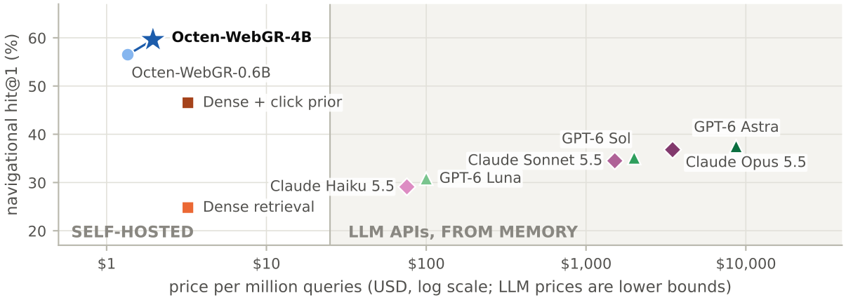
Generative retrieval has stayed below ten million documents; the largest public experiment is the 8.8 million passages of MS MARCO. The Octen team's Octen-WebGR (a model that does web navigational search with generative retrieval) pushes it to 201 million web pages. Every page is named by two tokens; a 4B-parameter model reads the query, generates the two tokens directly, and a table lookup returns the URL. On real navigational traffic from the month after training ended, it ranks the target page first 59.6% of the time, against 46.5% for a dense retriever trained on the same clicks and reranked by click counts, and at most 37.5% for frontier LLMs answering from memory. Serving needs one GPU and about 10 GB of memory, while the exact dense index needs 412 GB.
Search and recommendation retrieval teams should read it closely, not because "generative retrieval wins" but because it measures the division of labour between the two families very clearly. For a page that already has many clicks, searched with a new phrasing, generative retrieval ranks it first 30.9% of the time and dense retrieval 17.2%. For rarely clicked pages the order flips: dense retrieval 24.3%, generative retrieval 14.3%. The core idea in one sentence: writing each page's click history into the model's weights lets it learn a preference term that depends on the page alone, which similarity search cannot provide. The evidence comes from proprietary click data, the dense baseline trains only two linear layers, and there is no online experiment; keep these in mind when reading the conclusions.
What problem is it actually solving?
Many searches do not ask a question; they name a page. A user typing "nyt connections" wants the New York Times word puzzle page, and only ranking it first counts. Such navigational queries are answered today mainly by two tools, each with a blind spot.
| Method | How it answers | Blind spot (illustrative) |
|---|---|---|
| Click table | returns the page past users clicked most for the same query | a new phrasing such as "new york times connections game" is not in the table, so no answer |
| Dense retrieval | embeds query and pages, returns the most similar | the site's help page, login page and other-language versions look alike and often rank above the target |
The paper's data show both blind spots are large. In September navigational traffic, 33.1% comes from queries never seen in training, which the click table cannot answer at all. Dense retrieval has the target in its top ten but not first for 30.8% of navigational traffic, and in 46.1% of those cases the page ranked above is another page of the same site. Generative retrieval aims to cover both: generalise to new phrasings, and learn which page users actually want.
Overall flow: two tokens name a page
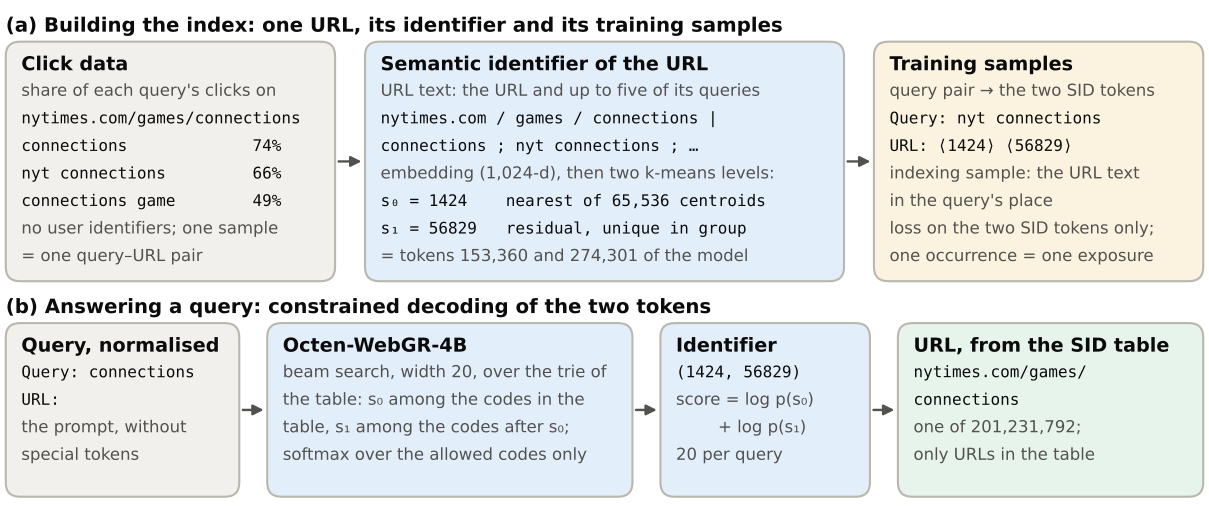
The system has three steps: assign every page a code, train the model on click data to generate codes, and decode under the code table at query time.
Step one: a unique code for each of 200 million pages
Why two tokens? Shorter codes mean fewer decoding steps, and two levels of 65,536 values give over four billion combinations, plenty for 200 million pages. The code comes from the page's "URL text": the normalised URL plus up to five of its most-clicked queries, such as "nytimes.com / games / connections | connections ; nyt connections ; …", with no page content. This text is embedded into a 1,024-dimensional vector, and two rounds of k-means follow. The first round clusters into 65,536 groups and the group index is the first code; the second clusters the residuals, vector minus centroid, into 65,536 groups to give the second code.
Plain two-round clustering has a flaw: two pages can land on the same pair. By the paper's count, 51.5% of 100 million pages would collide with another. The authors assign second codes within each first-level group in rounds: every unassigned page proposes its next-nearest residual centroid, and when several pages claim the same code, the closest keeps it. Every page ends with a unique code; 63.5% get their nearest centroid and 96.2% one of their nearest eight. Collisions are solved, at the cost of a few pages sitting slightly off their best position. Hoot says

Swipe or use the arrows for the three steps. Pages P, Q, R, centroids c1–c3 and the distances are illustrative; the paper gives no step-by-step example. The rule (each unassigned page proposes its next-nearest centroid; when several claim one code the closest wins) is from the text. The paper reports 63.5% of pages getting their nearest centroid. Source: paper §2: two k-means rounds of 65,536 clusters; plainly 51.5% of 100 million pages collide; within each first-level group second codes are assigned in rounds, each unassigned page proposes its next-nearest residual centroid and the closest claimant wins; all unique, 63.5% nearest, 96.2% within the nearest eight
The paper's example is nytimes.com/games/connections with code (1424, 56829). Each level has its own set of new tokens appended after Qwen3's 151,936 tokens, so first code 1424 is token 151,936+1,424=153,360 and second code 56829 is token 151,936+65,536+56,829=274,301. New token vectors are initialised as follows: for first code 1424, collect all queries that lead to pages whose first code is 1424, feed each as a prompt, take the final-layer hidden state the model uses to predict the next token, and average these vectors dimension by dimension. So from the start the model leans toward this code after similar queries.
Step two: training on clicks
A training sample is one pair of query and clicked page, written as "Query: q URL:" followed by the two code tokens, with loss only on the two code tokens. The sampling weight is the pair's share of the query's clicks times the square root of the query's total clicks. Why the square root? A query with 100 clicks, 80 on one page, gets weight 0.8×10=8; a query with ten thousand clicks, 8,000 on one page, gets 0.8×100=80. A hundredfold click gap becomes a tenfold sample gap, so popular queries are seen more without crowding out the long tail. Training also mixes in indexing samples: the page's URL text takes the query's place, with the page's two codes as the target. Since the URL text lists the page's most common queries, one such sample shows the model several phrasings at once.
Step three: only existing codes at query time
The normalised query becomes the prompt, and the model generates the two tokens by beam search of width 20. All valid codes form a prefix tree: the first step allows only first codes that occur in the table, the second only second codes that follow the chosen first code. Every result therefore maps to a real URL, and the model cannot invent addresses.
Main results: ahead overall, strong on new phrasings, weak on rare pages
| System | All navigational traffic | Seen pairs (62.0%) | New query, familiar page (9.0%) | New query, rare page (5.5%) |
|---|---|---|---|---|
| Octen-WebGR-4B | 59.6 | 88.2 | 30.9 | 14.3 |
| Dense retrieval (exact) | 24.8 | 34.4 | 17.2 | 24.3 |
| Dense + click rerank | 46.5 | 68.7 | 21.4 | 13.1 |
| BM25 (classic keyword retrieval) | 9.1 | 10.8 | 9.2 | 25.5 |
| Click table only | 58.9 | 93.4 | 0.0 | 0.0 |
Numbers are hit@1, the share of traffic whose target is ranked first, in %; a "familiar page" has at least 11 training queries pointing to it.
Overall, generative retrieval leads dense retrieval by 34.8 points, which shows that in navigation "which page" matters more than "how similar". With click reranking, the gap narrows to 13.0 points. The rerank takes dense retrieval's top 100 and scores each page as cosine similarity plus 0.04 times log10(1 + the page's training clicks). This means what dense retrieval mainly lacks is a score term that depends on the page alone, and generative retrieval learns that term into its weights from clicks. On the traffic where dense retrieval has the target in its top ten but not first, generative retrieval ranks it first 81.5% of the time, so it fills exactly the gap where other pages of the same site steal the top spot.
The last column flips: rare pages have only 1 to 10 training queries, generative retrieval has little to learn from, and dense retrieval and BM25 do better from the text similarity itself. The authors therefore tried a combination. The click table goes first. For queries not in the table, look at the first page generative retrieval returns: if that page has at least 3 training queries pointing to it and the model gives it a probability of at least 0.15, use generative retrieval's result, otherwise use dense retrieval. Both thresholds were chosen on the July development set. Overall hit@1 reaches 63.1%, showing that a simple router can combine the strengths of both.
More pages hurt generative retrieval far less
This experiment does not retrain the model; it only restricts candidates at query time. The authors draw nested random subsets of 2M, 8M, 32M and 128M pages from the 201M, each first seeded with every target page of the September evaluation traffic and its same-site pages, then filled at random. Generative retrieval decodes only over the subset's prefix tree, and dense retrieval searches only the subset. From 2 million to 201 million, generative retrieval's hit@1 falls only from 64.2% to 59.6%, 4.7 points; dense retrieval falls from 47.0% to 24.8%, 22.2 points. The two treat added pages differently: for dense retrieval each extra page is one more distractor that may happen to look like the query; generative retrieval has concentrated probability on pages users click, so most added pages never reach the top ranks.
On cost, the 4B model uses 9.7 GB of GPU memory, about 2.3 ms of GPU time per query in batches of 64, and 56 ms single-query latency; the 0.6B version even runs on one CPU socket at 72 ms per query. This shows its serving cost is comparable to inference of a mid-sized language model, without maintaining a huge vector index for 200 million pages. Figure 1 shows that LLMs answering from memory are not only less accurate but cost at least 40 times as much per million queries.
The bottleneck is exposure, not model size
The most interesting part of the paper analyses how much generative retrieval can remember. Fixing each query-page pair at exactly two training exposures, the authors compare models from 0.6B to 14B. Larger models learn more per exposure, but the real limit is how often and when a pair is seen: the same 0.6B model trained 16 times per pair ranks 67.4% of trained pairs first, beating the 14B model trained twice (64.3%), with about a quarter of the compute.
Repetition does not help new queries, though. On 4,000 navigational queries withheld from training, raising the same pairs from 2 to 16 exposures lowers hit@1 from 17.9% to 14.5%, almost back to the 13.7% before training. Spreading the same 16 samples over 16 different queries of a page, once each, is what helps new queries. This means scaling generative retrieval is a matter of training schedule: each page must be seen through many different phrasings, and late in training while the learning rate decays, or later samples wash out what was learned early.
Limitations as I see them
First, the baselines are weak. The authors admit the dense baseline trains only two linear maps on a frozen encoder, with about 2% of generative retrieval's training compute, and BM25 is untuned. A dense model fully fine-tuned on the same click pairs might narrow the 34.8-point gap considerably.
Second, the gain next to a click table is small. Production systems usually query the click table first, and in that setup generative retrieval adds only 0.7 points of hit@1 over a dense fallback, and routing another 0.6. For a search system that already has a mature click table and dense retrieval, the real increment is these one or two points, not the 34.8 in the table.
Third, data and evaluation cannot be reproduced. The click data are proprietary, every configuration was run once, and there is no online experiment; the only public evaluation uses Bing clicks six years older. Over half of new-query targets are not among the 201 million pages at all, and no system can answer those.
How a recommendation or search team could try it
- Confirm the scenario first: pick queries whose clicks concentrate on one result. These navigational requests are where generative retrieval is strongest; in recommendation the analogue is searches for one specific product or account.
- Encode the candidate set with two rounds of k-means plus the round-based code claiming, and check the collision rate and the share of items that get their nearest centroid. This needs no model training.
- Train a small model on click pairs, with sampling weight equal to click share times the square root of the query's clicks, and add samples that combine many phrasings. Evaluate separately on seen pairs, new queries for familiar targets and new queries for rare targets.
- In production, do not replace existing retrieval; place it after the click table, in parallel with dense retrieval, and route with thresholds, sending rare targets to dense retrieval.
Verdict
For navigational retrieval, where there is one right answer from a fixed list and clicks to learn from, generative retrieval now scales to 200 million items and is cheap to serve; but what it fixes is dense retrieval's ranking weakness, and rare targets still need dense retrieval.
| Dimension | Assessment |
|---|---|
| Problem importance | High. Navigational queries are a fifth to a quarter of search traffic, and both click tables and dense retrieval have clear blind spots |
| Method novelty | Medium. Two-level semantic codes and constrained decoding exist; the novelty is the engineering to 200 million items and a systematic measurement of memorisation |
| Experimental evidence | Medium-high. Fine-grained block evaluation and scaling studies, but weak baselines, proprietary data and no online test |
| Engineering cost | Medium. One GPU serves it, but training the 4B model takes about a thousand GPU hours; deleting a page only needs removing it from the table, while adding pages needs further training |
| Worth trying | Worth trying as supplementary retrieval after the click table, validated first on navigational queries |
| Fit | Search with a single target, a fixed candidate set and abundant clicks, such as web navigation or direct product or account lookup |
How did this read for you?
Hoot made a note. Thanks for the feedback.

One tap, no sign-in; tap again to undo. Only anonymous counts are kept, never who you are.
Discussion
Add experiment details, reproduction notes or a different take. Requires a GitHub sign-in.
Loading the discussion…