 NeurIPS 2026
Contents · 7 sections
1How an annual report becomes 16 prefix tokens2Retrieving image tokens with a text question, through a projection trained with the compressor3Compressing 256 into 16, with the question added on both sides4Main results: ahead on raw score on LongBench-v2, behind on BAMBOO5The CAP multiplier: 16 tokens buy about 1.39x6Two ablations: 16 is the peak, and query-driven compression beats query-agnostic alternatives7Where this approach appliesSHARE

OpticalRAG renders a long document as page images and hands a frozen 7B model only 16 tokens, yet on LongBench-v2 it answers better than methods that read thousands of text tokens; but the combined score on which it ranks first on all three benchmarks comes largely from the fact that it uses only 16 tokens.
Start with the setting. Picture a 100,000-character English annual report (illustrative), and a four-way multiple-choice question: "In which year did R&D spending first exceed 15% of revenue?" A RAG system has to find the relevant content in the report, put it into the model's context, and let the model pick A/B/C/D. Feeding the whole report is too expensive, so something always gets compressed first.
The difficulty is that compression ratio and detail pull against each other. The answer may hinge on a single mid-report sentence, "R&D spending was 15.3% of revenue" (illustrative), plus one year. Compressed to a few thousand tokens, that sentence probably survives; compressed to a few dozen tokens, the model sees so little that keeping one specific number and its year becomes hard.
Existing methods fall into roughly two groups, and both go wrong on the report example. The first group deletes or rewrites text: LLMLingua-2 and Selective Context drop tokens they judge unimportant, and RECOMP (a retrieve-then-summarize compressor) rewrites retrieved passages into a summary. Under aggressive compression, the "15.3%" sentence may be deleted or summarized as "R&D investment kept growing", and no later step can bring deleted tokens back. The second group is xRAG, which encodes a whole document into one vector injected into the model; the year, the ratio and the context are all squeezed into that one vector, and the model struggles to read out "which year" again.
The authors start from an observation: a rendered page of text, passed through a modern visual encoder, turns the content of a few hundred text tokens into roughly a hundred visual tokens while keeping most of the meaning. So they move compression into pixel space: render the document as page images first, then retrieve and compress over visual tokens.
How an annual report becomes 16 prefix tokens
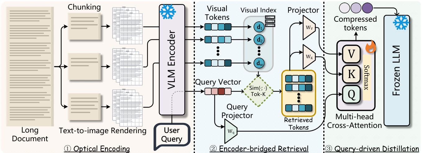
The paper splits the method into three stages, encoding, retrieval and distillation; with rendering at the start and answering at the end there are five steps. The table below follows the report example. The visual encoder and the language model stay frozen throughout; only the compressor and the final bridge MLP are trained.
| Step | Input | Operation | Output (report, illustrative) | Trained? |
|---|---|---|---|---|
| Render | 100,000 characters of text | Split sequentially into chunks of at most 24,000 characters; typeset each chunk into some number of 640x640 page images | 5 chunks, about 12 pages each, 60 pages total | No |
| Encode | 60 page images | The frozen DeepEncoder (the SAM plus CLIP visual encoder from DeepSeek-OCR) outputs 100 visual tokens of 1024 dimensions per page | 6,000 visual tokens, each stored in this document's inner-product index | No, done offline |
| Retrieve | Question, options and instruction | Run the question through the frozen LLM, take last-layer hidden states, project into visual space with linear map W_q, max-pool into one query vector, take the top 256 by inner product | 256 visual tokens, sorted by original position | W_q is trained |
| Distill | 256 visual tokens plus the query vector | Reshape into a 16x16 grid and downsample to 64 with a depthwise convolution; 16 learnable "compression slots" read from these 64 via cross-attention; an MLP projects into the LLM input space | 16 soft prefix vectors of 3584 dimensions | Trained |
| Answer | 16 prefixes plus the question text | The prefix is placed before the question's text embeddings; the frozen Qwen2.5-7B scores A/B/C/D | One option | No |
So the document content the model finally sees occupies only 16 positions. The question, options and instruction still go in as text (truncated to 1,024 tokens), and that part does not count toward the 16-token budget.
Retrieving image tokens with a text question, through a projection trained with the compressor
The first problem is a modality mismatch. The report has become 6,000 visual tokens, while the question is a piece of text. The authors stress that they do no contrastive training and no end-to-end cross-modal alignment training, which they regard as costly.
OpticalRAG skips contrastive training. The question first goes through the frozen Qwen2.5-7B; the last-layer hidden state at each position is mapped by a linear projection W_q into the space where the visual tokens live. To get a single query vector, a max is then taken over all positions. This vector is dotted with each of the 6,000 visual tokens, and the top 256 are kept.
W_q has no retrieval loss of its own. It belongs to the compressor and is trained jointly with the distillation step. In other words, W_q is trained so that its projected vector is useful for compression, and retrieval simply reuses it for scoring.
The intermediate product of this step looks like this (illustrative): one 1024-dimensional query vector plus a 256-row list, each row a visual token and its position in the original, such as page 3 token 41, page 17 token 8, page 18 token 62, and so on. The list is sorted by position before it goes to the next step. If retrieval works, the page carrying "15.3%" should contribute several tokens.
There is a boundary here that bears directly on the conclusions: how the number 256 was chosen. The authors state in the appendix that K=256 was chosen using feedback from the evaluation benchmark and should not be read as a hyperparameter chosen independently of it.
Compressing 256 into 16, with the question added on both sides
Why not prepend the 256 visual tokens to the model directly? Because the paper is after a tiny context budget. Also, visual tokens are not in the LLM's input space to begin with, so some layer has to translate them anyway. The authors make translation and compression the same step.
Compression begins with downsampling. The 256 retrieved tokens, sorted by position, are rearranged into a 16x16 grid and passed through a depthwise convolution with stride 2, which reduces them to 64 tokens. This grid only lays the retrieved results out in order as a square; neighboring cells are not necessarily neighbors on the original pages.
Next comes Q-Former-style cross-attention. The model holds 16 learnable vectors, which can be thought of as 16 "compression slots". Through two layers of cross-attention, each slot distributes attention weights over these 64 downsampled tokens and reads content in by those weights. After reading, the slots go through a two-layer MLP into the LLM's input dimension, so they can serve directly as a soft prefix placed before the question.
The query vector is used twice here: it is added to every visual token, and also to the initial value of every compression slot. Adding it only on the token side is not enough, and the reason can be worked out mentally (illustrative). Suppose a slot scores two tokens at 3 and 1. Adding the same query vector to both tokens raises both scores by the same amount, say 2 each, giving 5 and 3. Softmax only looks at score differences, so this slot's attention does not change at all. Only once the slot itself carries the query vector can different questions make the same slot look at different tokens. This is the point the authors discuss in Appendix A.4. Hoot says

Question added to tokens only (illustrative)
- slot score for token A
- 3 → 5
- slot score for token B
- 1 → 3
- gap A − B
- 2 → 2
- read-out split A : B
- 88% : 12%, unchanged
Both scores gain the same amount; softmax cancels it
Slot also carries the question (illustrative)
- slot score for token A
- 3 → 4
- slot score for token B
- 1 → 5
- gap A − B
- 2 → −1
- read-out split A : B
- 27% : 73%, flipped
The slot changed, so each token gains differently; a different question reads a different token
Illustrative numbers: one compression slot, two visual tokens, read-out split = softmax over the two scores. Adding the same question vector to every token passes through a linear key projection, so the slot's score for every token rises by the same amount; softmax only sees differences, so the split does not move. Once the slot itself carries the question vector, its dot product with each token changes by a different amount, so the gap can follow the question. All of this happens in the visual space; only afterwards does a separate bridge MLP project the slots into the LLM input space, and the two modules are merely trained together. The authors' theorem rests on this step: assuming each needed piece of evidence has one clearly winning best token and the answer depends on only a few directions of those tokens, having at least that many slots makes compression nearly lossless.
Source
paper §4.3 (query vector added to tokens and to slots; bridge MLP); Appendix A.4 (token-side addition shifts all of a slot's logits by one constant, leaving softmax weights unchanged); §5 theorem assumptionsBack to the report example: each 2x2 block of retrieved tokens in the grid merges into one, so 64 remain after downsampling; the 16 slots read from these, about 4 per slot on average. But attention need not be spread evenly; ideally one slot puts most of its weight on the few tokens carrying "15.3%" and another locks onto the year.
The compressor and bridge MLP are trained in two stages. Stage one does reconstruction on Wikipedia and C4: a passage is rendered, encoded and compressed into a prefix, and the frozen LLM must reproduce the original text from the prefix. Stage two computes loss only on answers over SQuAD v2, DROP (a reading comprehension set that needs numerical reasoning) and CoQA, with early stopping on a dev set.
Why are 16 slots enough? The authors give a theorem: under several assumptions, as long as the number of slots is at least the number of independent factors the answer distribution depends on, compression can get arbitrarily close to lossless, regardless of how many tokens were retrieved. "Multiple-choice questions usually depend on only a few factors" is the authors' explanation for why 16 suffices, not a measured number.
Main results: ahead on raw score on LongBench-v2, behind on BAMBOO
Evaluation uses multiple-choice questions only: all 503 questions of LongBench-v2, plus the choice subsets of BAMBOO (a long-text understanding benchmark) and LooGLE-v2 (another long-document understanding benchmark). All methods share Qwen2.5-7B-Instruct as the backbone and answer by the next-token score over A/B/C/D; random guessing gets about 25%.
There are five comparison groups. The closed-book backbone gets no document and answers from the model's own knowledge. Standard RAG retrieves text chunks and puts them into the context. Selective Context, LLMLingua-2 and RECOMP are the text compressors described above, and xRAG is single-vector injection. The length column below is the number of document tokens fed to the model per question; CAP is the authors' combined score, unpacked in the next section.
| Method | LongBench-v2 score / length / CAP | BAMBOO score / CAP | LooGLE-v2 score / CAP |
|---|---|---|---|
| Closed-book backbone | 30.62 / 0 / 30.62 | 56.75 / 56.75 | 20.76 / 20.76 |
| Standard RAG | 31.41 / 1623 / 34.71 | 69.50 / 79.50 | 23.24 / 25.69 |
| Selective Context | 32.40 / 5512 / 33.69 | 70.00 / 74.85 | 22.49 / 23.44 |
| LLMLingua-2 | 28.23 / 2669 / 28.23 | 73.50 / 81.12 | 22.79 / 24.39 |
| xRAG | 26.24 / 1 / 26.24 | 51.00 / 51.00 | 21.06 / 32.54 |
| RECOMP | 32.01 / 6954 / 32.90 | 75.50 / 81.80 | 22.56 / 23.18 |
| OpticalRAG | 35.79 / 16 / 49.68 | 61.00 / 84.67 | 23.54 / 32.67 |
On LongBench-v2, OpticalRAG reaches 35.79 with 16 tokens, 5.17 points above the closed-book backbone and 3.4 points above the best text baseline, Selective Context at 32.40, which uses about 5,500 tokens. This shows that on this benchmark it gets a higher raw score than the text methods while using only 16 prefix positions.
On BAMBOO the picture flips. OpticalRAG's 61.00 is 8.5 points below standard RAG's 69.50 and 14.5 points below RECOMP's 75.50. The authors also acknowledge that RECOMP and LLMLingua-2 score higher on raw accuracy by keeping hundreds to thousands of text tokens. This shows that on BAMBOO, the information lost in the 16-token prefix is enough to leave accuracy clearly behind.
On LooGLE-v2, OpticalRAG's 23.54 is only 0.30 above standard RAG's 23.24, and every method sits within two or three points above the closed-book 20.76. This shows that raw scores barely separate methods on this benchmark, so the ranking is decided mostly by CAP.
The CAP multiplier: 16 tokens buy about 1.39x
So why is OpticalRAG still first on CAP on BAMBOO despite a raw score 14.5 points lower? That depends on how CAP is computed. The authors set the closed-book backbone's budget to B0 = 12k, the truncation length used for Qwen2.5-7B-Instruct, and give each method a compression multiplier:
For the other methods, B counts only document context tokens, not the question or options. The closed-book backbone is counted at B0, so its multiplier is 1 and its CAP equals its raw score; the 0 in its length column only means it gets no document, not that its multiplier is computed with B=0. When a score is at least the closed-book score, CAP is the score times m(B); below it, CAP is just the score, with no compression credit.
Because the exponent 0.05 is small, the multiplier grows slowly: 10x compression gives about 1.12, 100x gives about 1.26. Sixteen tokens amount to over 700x compression, so the multiplier is about 1.39.
Now work out BAMBOO. RECOMP uses about 2,400 tokens, a multiplier of about 1.08, so its CAP is about 81.8. OpticalRAG is 61.00 times 1.39, about 84.7, matching the 84.67 in the table. This shows that the 14.5-point raw-score gap is overturned by the difference in multipliers.
OpticalRAG's first place on CAP on BAMBOO and LooGLE-v2 comes mainly from the roughly 1.39x multiplier that 16 tokens earn, not from answering more questions correctly.
The same logic is even plainer for xRAG. xRAG uses 1 token, with a multiplier of about 1.55; its 21.06 on LooGLE-v2 is just above the closed-book 20.76, so its CAP jumps to 32.54, almost level with OpticalRAG. The authors themselves note that xRAG's CAP is propped up by the multiplier. The same criticism applies to OpticalRAG's 32.67 on LooGLE-v2. On average CAP across the three benchmarks, OpticalRAG has 55.67 and the runner-up, standard RAG, has 46.63, and that gap needs to be unpacked the same way.
On LongBench-v2 and LooGLE-v2, OpticalRAG leads on both raw score and CAP, though on LooGLE-v2 its raw lead is only 0.30 points; on BAMBOO it leads only on CAP. LongBench-v2 is also the benchmark whose feedback informed K=256.
Two ablations: 16 is the peak, and query-driven compression beats query-agnostic alternatives
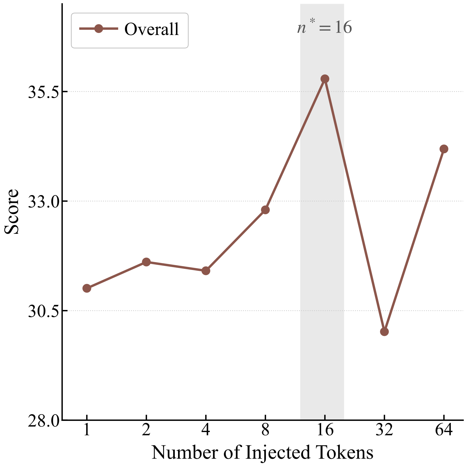
The first ablation varies the number of compression slots from 1 to 64. Scores mostly rise from 1 to 16, with 16 the best; 32 drops sharply, and 64 partly recovers and is best on long examples. The authors read this as the slot count needing to balance evidence coverage against noise. This shows that more slots are not always better, and 16 is the measured peak of this curve.
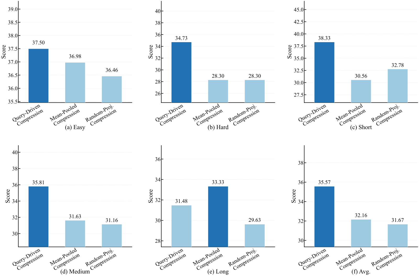
The second ablation fixes the budget and compares query-driven compression with two compressors that ignore the question: one mean-pools the retrieved tokens, the other uses a random projection. On LongBench-v2 the three score 35.57, 32.16 and 31.67. In other words, query-driven compression is about 3.4 and 3.9 points above the two query-agnostic alternatives. But both controls also replace the cross-attention compression structure, so these numbers cannot isolate the effect of adding the question to the compression slots.
Where this approach applies
Back to the report example. If the question becomes "How did the R&D share change over the past five years?", the answer needs one number from each of five widely separated years. The authors write in their limitations that a fixed prefix budget may not suit questions that need evidence from several distant segments, and this is exactly such a question.
A few more points affect how to read the results. The 16 tokens count only the visual prefix; the question, options and instruction are input separately. The length column also excludes the offline compute for rendering, encoding and indexing. The evaluation covers only multiple-choice questions and a single 7B backbone; open-ended generation is left for later.
The paper establishes one concrete thing: a frozen OCR visual encoder plus a small compressor can squeeze a long document into 16 prefix tokens and still lead on raw score on LongBench-v2. As for "first on CAP on all three benchmarks", divide out the 1.39x multiplier before reading it.
How did this read for you?
Hoot made a note. Thanks for the feedback.

One tap, no sign-in; tap again to undo. Only anonymous counts are kept, never who you are.
Related papersMore from Paper Daily
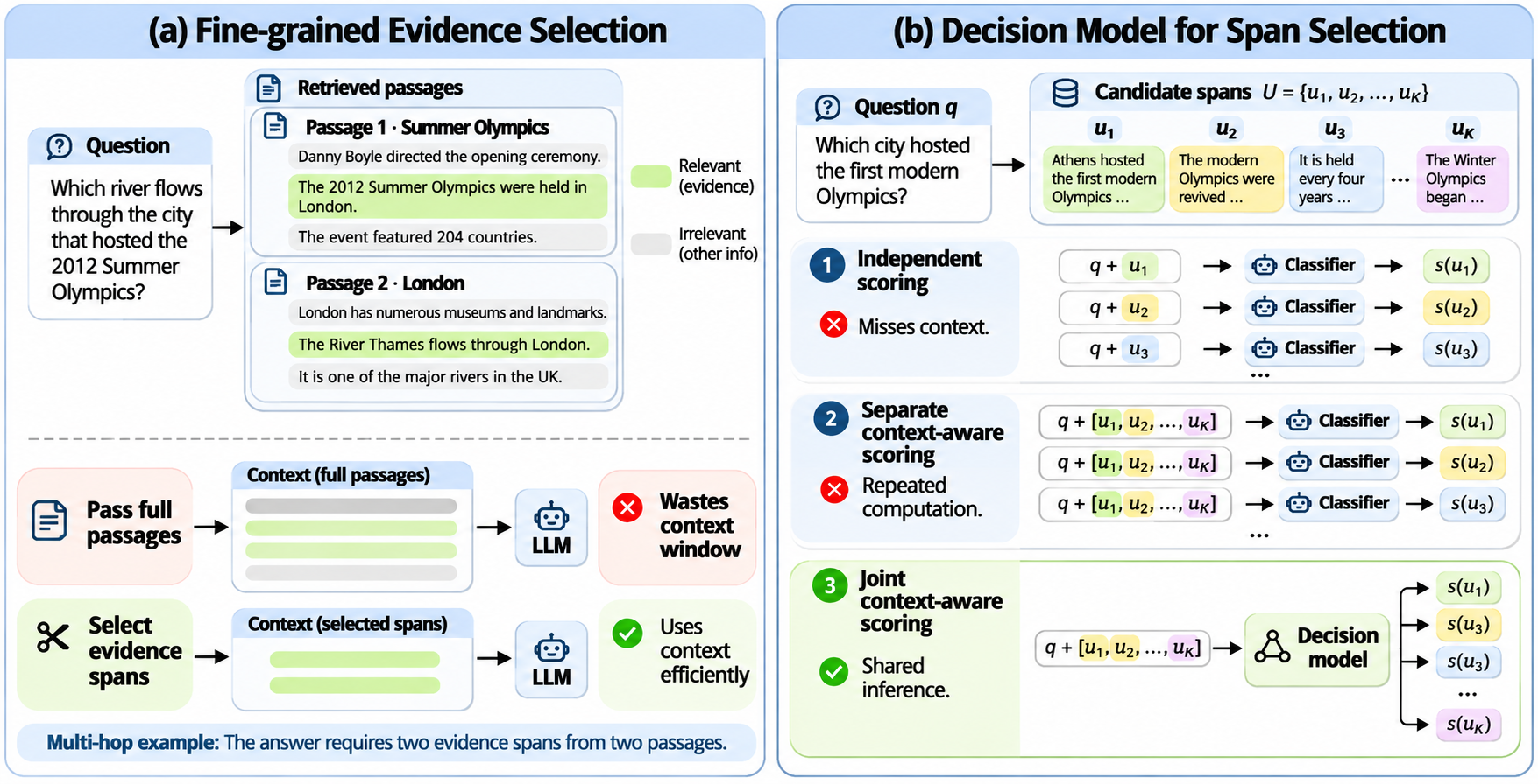 Retrieval · 2026-11-16CURATOR: Scalable Fine-grained Evidence Selection for Retrieval-Augmented Generation using Decision ModelsRAG usually stuffs whole retrieved passages into the LLM, though often only a few sentences in them can answer the question. Picking those sentences is not easy: a sentence can look irrelevant on its own, and whether to keep it may depend on other retrieved text. Judging each sentence with the full context is too expensive. Decision models can score many candidate sentences in one pass, with each…
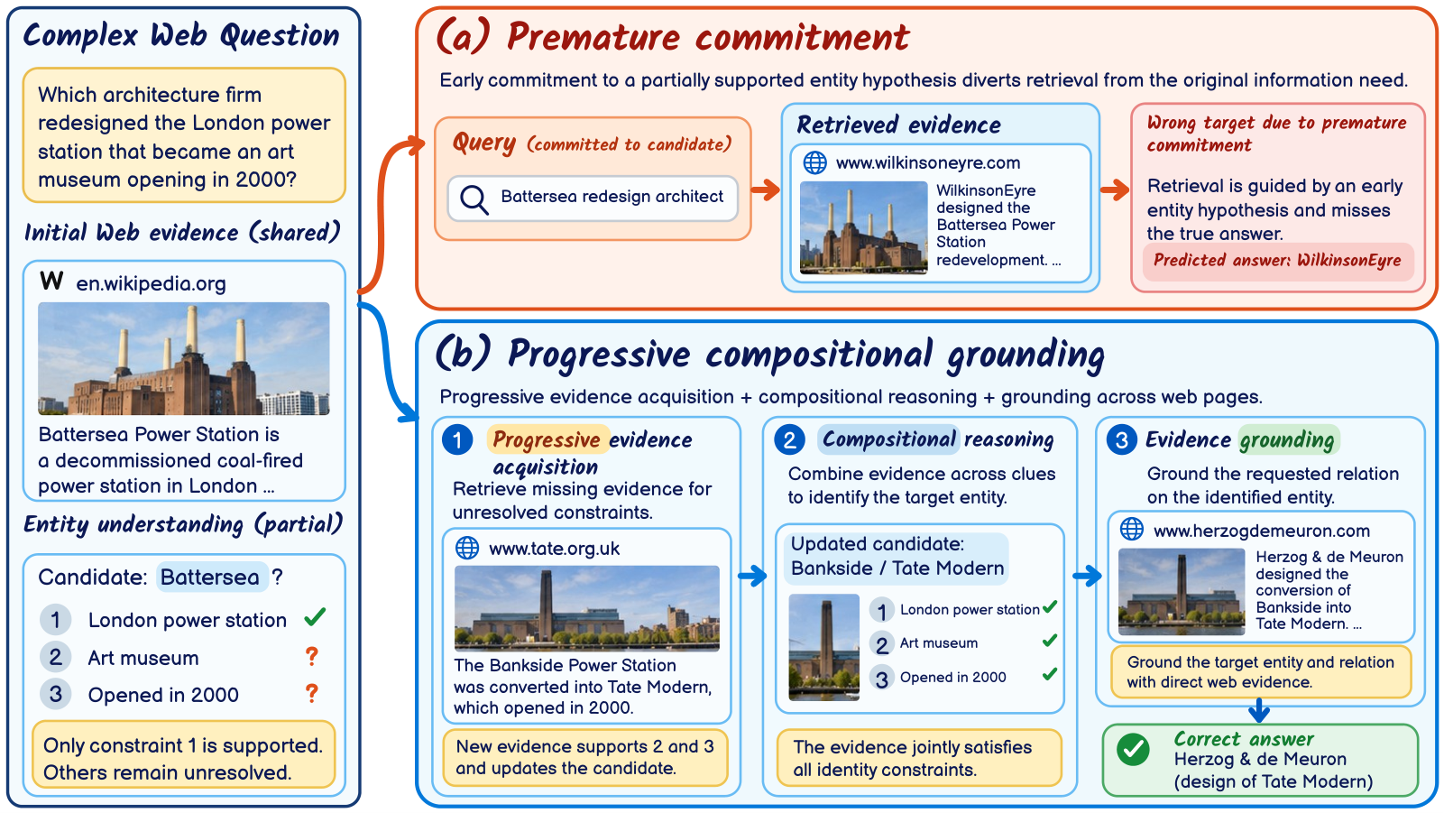 Retrieval · 2026-11-13PCG-RAG: Progressive Compositional Grounding for Retrieval-Augmented Generation in Complex Web Question AnsweringComplex web QA often requires first working out who or what several clues describe, then looking up an attribute of it, and a common mistake is to treat a name as settled after only one clue matches. The paper's example is a London power station converted into an art museum: a system that settles on Battersea from London and power station alone retrieves an architect who actually belongs to a dif…
 Retrieval · 2026-11-11Lightfoot: Graph Retrieval-Augmented Generation with Exact, Model-Free Document DeletionGraphRAG in production has two costs that papers rarely count: what it takes to build the graph, and how painful it is to delete a document. When a contract expires or a user asks for erasure, a document and everything derived from it must go, yet entity summaries that blend several documents are hard to take apart. Lightfoot requires every record in the graph to be computed only from single-pass…
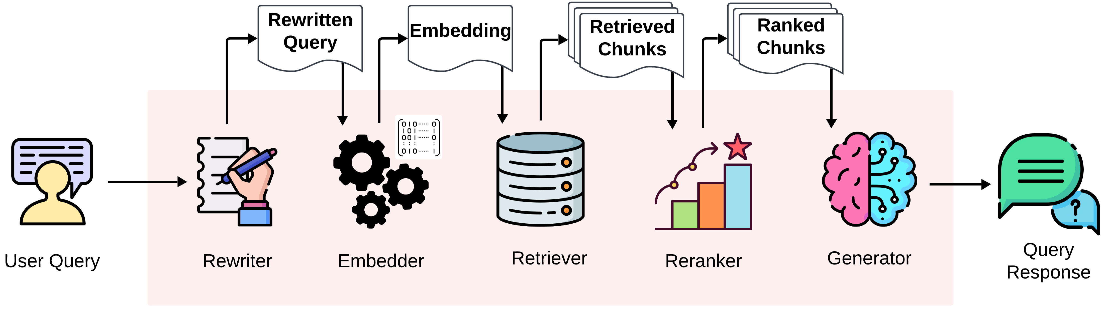 Retrieval · 2026-11-05From Logs to Faults: Reference-Free Fault Localization for Retrieval-Augmented Generation PipelinesRAGLog reads only the API logs each run of a RAG pipeline leaves behind, with no reference answers and no code changes, and points out which stage of the run went wrong. This matters because a pipeline can go wrong in the middle and still give the right final answer. Across natural runs of five open-source pipelines, 37% had at least one faulty stage, and more than a third of those still answered…
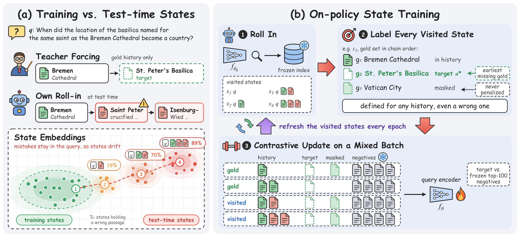 Retrieval · 2026-11-02Retrieving from Your Own Mistakes: On-Policy Training of Embedding Models for Multi-Hop Retrieval-Augmented GenerationChain embedding retrievers for multi-hop retrieval see different histories in training and in use, and this paper fixes that without adding any LLM call. At each step such a retriever joins the question with the passages found so far to look for the next one; in training its history holds only correct passages, but in use it often holds wrong passages it found itself. On four-hop MuSiQue question…
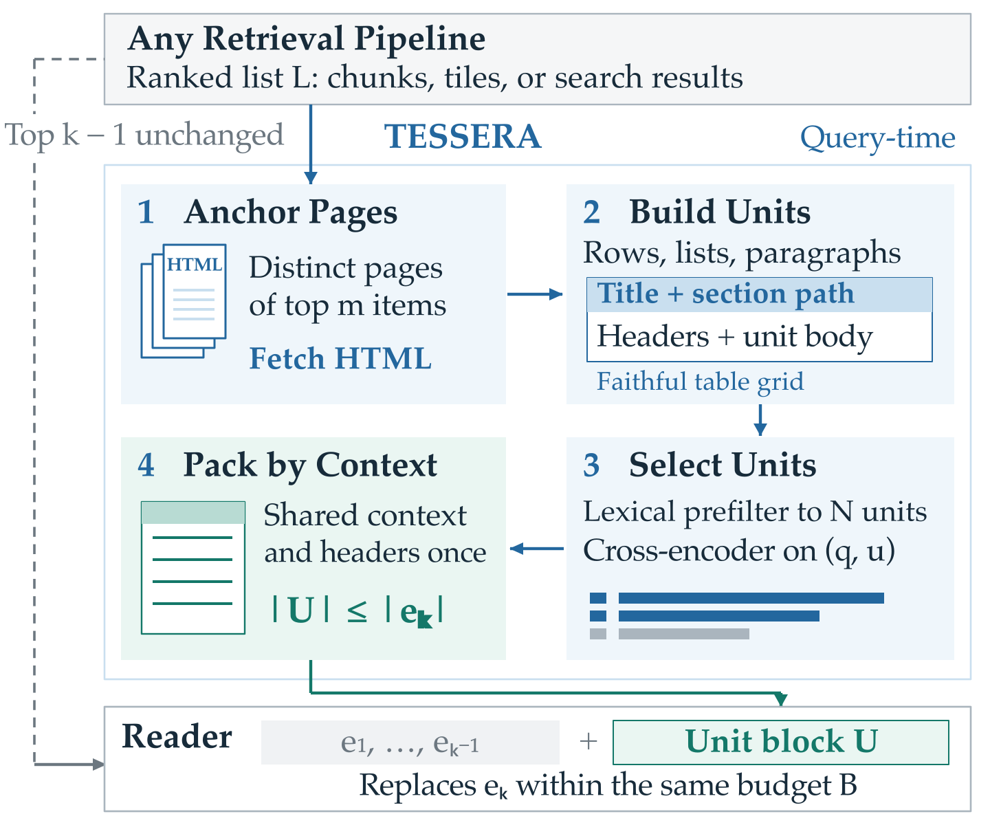 Retrieval · 2026-10-29Tessera: Structure-Completed Evidence Units for Web Retrieval-Augmented GenerationAsk Wikipedia who produced Willy Wonka and the Chocolate Factory, and the answer sits in the producer row of the page's infobox. Text extraction drops the two names in that cell, the reader model sees only the director, and it answers wrong. Tracing answer evidence from page source to reader input over all of English Wikipedia, this paper finds such loss is common: for 7.6% of questions the evide…
 Retrieval · 2026-11-04DR Pixel: Page-Native Deep Research with Vision-Language ModelsLetting a research agent read page screenshots, instead of first converting PDFs to text and searching that, raises question-answering accuracy and needs fewer searches. DR Pixel renders about 1.06 million paper pages as images and encodes each image as one vector. The agent issues text queries, gets back the most relevant page images, and keeps looking at these original images for the whole traj…
Discussion
Add experiment details, reproduction notes or a different take. Requires a GitHub sign-in.
Loading the discussion…