SHARE

Perplexity has released two multi-vector retrieval models, pplx-embed-v2-late, at 0.6B and 9B parameters, which encode text, images and screenshots of document pages. They are "late-interaction" retrievers: every document token is stored as a 128-dimensional vector, every query token also gets its own vector, and scoring takes, for each query vector, the largest inner product with any document vector, then sums those maxima (MaxSim). The two models are not trained separately with contrastive learning. Instead both imitate, token by token, the vectors produced by the same 18B teacher, so they land in the same embedding space: a document collection can be indexed offline with the 9B model and queried online with the 0.6B model, scoring directly. On 72 domain retrieval tasks assembled by the authors, the 9B model averages 81.3% nDCG@10, 1.6 points above the runner-up nemotron-3-embed-8b. A 0.6B query against a 9B document index scores 79.6%, 1.6 points above using 0.6B on both sides, at the same query-side cost. This is a short technical report, and the credibility of its main results has to be judged piece by piece. The task list of the domain benchmark is not public, and the labels of the two production benchmarks partly come from Perplexity's own production system; only ViDoRe-V3 and BrowseComp+ can be reproduced independently.
1. Why late interaction, and why distillation
Retrieval models usually trade off between two designs. Single-vector models compress a whole document into one vector, which is fast with approximate nearest-neighbor search but loses detail. Cross-encoders run the query and document through the model together, which works well but needs a separate pass per candidate, so they are only usable for reranking. Late interaction sits in between: document token vectors are computed offline and stored, at query time only the query's vectors are computed, and MaxSim does the scoring. The price is storage, which is why this work compresses each token vector to 128 dimensions.
The authors' other judgment is that small models trained directly with contrastive learning fall short, and fitting the token vectors of a large model works better, especially at small sizes. A by-product is that students of different sizes distilled from the same teacher are interchangeable. The report body, however, gives no numbers comparing distillation with direct contrastive training, so for now this is the authors' experience only.
2. Training pipeline
2.1 The 18B teacher: two-stage contrastive learning
The teacher is Qwen3.5-27B with its last 20 layers pruned, giving 18B, and with the causal mask removed from the attention layers so every token sees both sides of its context. Training has two stages.
The first stage uses query–document pairs. The data come from 28 datasets, further split by language and domain into 981 subsets, 186M pairs in total. 88.3% are text–text, 8.3% text–image and 3.4% text–document-screenshot, and 14M of the text pairs are synthesized by generating queries backward from PDF passages. Sampling weights are adjusted during training to change the three proportions to 56.5%, 30.9% and 12.6%, heavily upsampling images and screenshots. Each batch is drawn from a single subset, so the other documents in the batch (the negatives) are closer to the positive and harder to tell apart. To make subsets appear in their target proportions and at evenly spaced intervals, the authors do not draw independently at each step. They cut 0 to 1 into 981 segments, each as long as its subset's sampling share, with subsets from the same source placed next to each other. At step they take the fractional part of "random start " (0.618 being the inverse golden ratio), and the segment it lands in supplies that batch. These points cover 0 to 1 very evenly, so each segment is hit about as often as its length and the hits are spread out in time; subsets from one source form one long segment, so "proportional and evenly spaced" also holds at the source level. The contrastive batch is 16,384 pairs, trained with LoRA (rank 128). In-batch documents whose MaxSim score is within 0.2 of the positive's are not counted as negatives, to reduce false negatives. MaxSim is written as a Triton kernel to avoid materializing the token-level similarity matrix.
The second stage merges the LoRA weights, adds a new rank-32 adapter, freezes the vision part and trains on text triplets only: each query gets one positive and up to 4 hard negatives. Some hard negatives are synthesized by changing key information in highly templated documents, for instance a financial report in a fixed format with a single number changed, which forces the model to read details.
2.2 Students: fitting the teacher's vectors token by token
The student loss is direct. For every valid query and document token, take the Euclidean distance between the student vector and the teacher vector (both L2-normalized), average the query part and the document part separately, and add them. The teacher is not updated.
Because this loss does not rely on in-batch negatives, a batch can mix several subsets, which steadies the gradient. The 9B student is based on Qwen3.5-9B. The authors found LoRA alone could not fit well enough, and they guess that token-level alignment constrains the whole embedding space too tightly. So they fully fine-tune the last 8 layers of the text part and use LoRA elsewhere. The 0.6B student is pruned from Qwen3.5-0.8B, removing 2 of the 3 linear-attention (Gated DeltaNet) layers in each block. It ends up with 594M parameters in total, of which 254M are the token-embedding table and 100M the image encoder, so about 240M are actually active for text. It is fully fine-tuned, because full fine-tuning clearly beat training adapters only on document-screenshot tasks.
3. Experiments
3.1 Text retrieval
The domain benchmark consists of 72 public tasks covering finance, legal, health, conversation, tech and multilingual, with task counts ranging from 4 in tech to 20 in legal. The metric is nDCG@10, averaged with equal weight over the six domains:
| Model | Dim | Avg | Finance | Legal | Health | Conv. | Tech | Multiling. |
|---|---|---|---|---|---|---|---|---|
| pplx-embed-v2-late-9b | 128 multi | 81.3 | 82.5 | 81.6 | 82.5 | 81.5 | 70.4 | 89.5 |
| nemotron-3-embed-8b | 4096 single | 79.7 | 80.8 | 81.1 | 83.9 | 77.4 | 67.5 | 87.9 |
| voyage-4-large | 1024 single | 79.0 | 81.5 | 80.0 | 83.0 | 76.7 | 65.1 | 87.9 |
| pplx-embed-v2-late-0.6b | 128 multi | 78.0 | 79.9 | 78.2 | 78.0 | 79.7 | 66.6 | 85.8 |
| voyage-4-nano | 2048 single | 74.6 | 77.3 | 75.8 | 76.0 | 74.7 | 59.4 | 84.3 |
| qwen3-embedding-0.6b | 1024 single | 68.4 | 67.9 | 70.0 | 72.4 | 68.4 | 53.9 | 77.8 |
The 9B model is best in every domain except health; the 0.6B model is best among sub-1B models in every domain. The 9B model's largest leads are in conversation (+4.1) and tech (+2.9), domains with only 5 and 4 tasks, where a single task's swing moves the average a lot. In legal, the domain with the most tasks, 9B is only 0.5 above nemotron. The authors withhold the task list so that later models cannot tune to it. The reason is understandable, but the cost is that this table cannot be checked.
Q2D-Web is closer to Perplexity's production setting: about 70,000 agent-rewritten production search queries over a corpus of 190M web pages, measured by Recall@1000. Relevant documents have three kinds of labels: documents the agent cited in its answer; documents the production retrieval system ranked high; and the union of those two, extended with documents an LLM judged relevant. The table compares the two pplx models with the strongest baselines:
| Model | Cited by agent | Ranked high by production system | Combined (plus LLM judgments) |
|---|---|---|---|
| pplx-embed-v2-late-9b | 88.2 | 68.8 | 74.8 |
| pplx-embed-v2-late-0.6b | 86.7 | 67.3 | 73.6 |
| nemotron-3-embed-8b | 83.1 | 61.7 | 69.3 |
| qwen3-embedding-8b | 79.3 | 58.3 | 65.3 |
The second column treats documents ranked high by Perplexity's production retrieval as relevant, which naturally favors models that rank like the production system, and the pplx models lead nemotron most in this column (7.1 points). The authors therefore emphasize the combined labels, which they say reduce this bias. But the first column, "documents cited by the agent", also comes out of the production system's search results and carries the same lean, so none of the three columns is fully neutral. Even so, the 0.6B model beats the 8B nemotron in all three columns, which shows the advantage is not all label bias.
The report also tests the text version of ViDoRe-V3, where document page screenshots are converted to Markdown by OCR before retrieval, again scored by nDCG@10. The 9B model scores 64.7%, the 0.6B 61.2%, and the best baseline, nemotron, 60.6%. This is the only text result that can be reproduced independently.
3.2 Document-screenshot and image retrieval
All three benchmarks below are text-to-image retrieval, scored by nDCG@10 (%).
| Model | Dim per token | ViDoRe-V3 (screenshots) | MIRACL-Vision | PPLX-Q2I |
|---|---|---|---|---|
| pplx-embed-v2-late-9b | 128 | 65.2 | 75.7 | 65.0 |
| pplx-embed-v2-late-0.6b | 128 | 62.3 | 67.5 | 60.4 |
| topk-embed-v1-2b | 128 | 61.9 | 60.2 | 51.5 |
| gemini-embedding-2 | 3072 (single vector) | 46.0 | 77.5 | 67.0 |
| qwen3-vl-embedding-8b | 4096 (single vector) | 58.3 | 68.5 | 50.6 |
| evie-8b (image retrieval only) | 4096 | 66.4 | – | – |
On images it does not lead across the board. On ViDoRe-V3, EVIE (a vision-only multi-vector model) trained specifically for image retrieval scores higher in both its 8B and 4.5B versions, at 66.4% and 65.9%. But they store 4,096 and 2,048 dimensions per token, while pplx-embed-v2-late stores only 128, so the gap has to be read together with storage cost.
The fairest comparison is topk-embed-v1, also at 128 dimensions: the 0.6B model is 0.4 points above the 2B topk model, while topk at its full 2,048 dimensions is 0.9 points above the 0.6B model. That means under the same storage budget, pplx's small model matches a model of the same kind with more than three times the parameters. On MIRACL-Vision (Wikipedia page screenshots) and PPLX-Q2I (Perplexity's production image-search logs, 10,000 queries and 100,000 images), gemini-embedding-2 scores higher. PPLX-Q2I defines relevant images as "images actually served in production", carrying the same production-system lean as Q2D-Web. EVIE and Nemotron ColEmbed were not evaluated on this set; the authors say their dimensions are too high to make indexing practical.
3.3 Small-model queries + large-model index
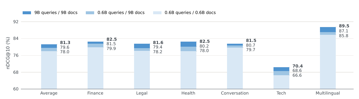
Documents are indexed with the 9B model, and queries are encoded with either 9B or 0.6B. A 0.6B query against 9B documents beats 0.6B on both sides in all six domains, raising the average from 78.0% to 79.6%; 9B on both sides scores 81.3%. In other words, switching only the document side recovers almost half of the 9B model's 3.3-point advantage over 0.6B. Query encoding costs the same as pure 0.6B, and the cost of indexing documents is amortized over the life of the index. The report runs this experiment only on the domain benchmark, not on Q2D-Web or the image tasks.
3.4 As the retriever for a search agent
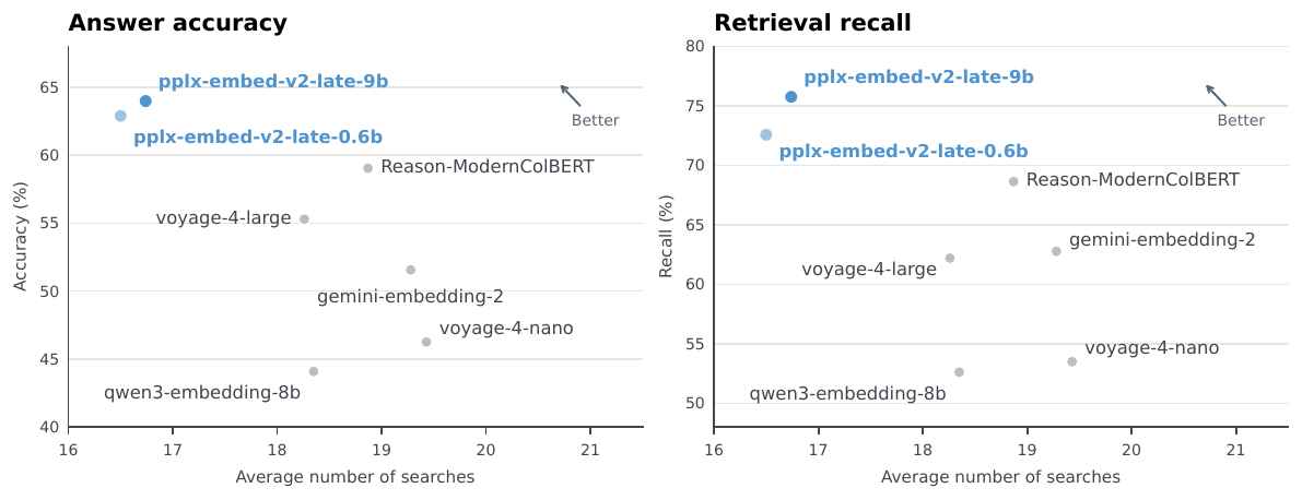
BrowseComp+ has GPT-OSS-120B act as an agent that repeatedly searches a fixed corpus with the retriever under test to answer complex questions, and another LLM grades the answers. The 9B model reaches 64.0% accuracy, 4.9 points above the other late-interaction model, Reason-ModernColBERT, and 8.7 points above the best single-vector model, voyage-4-large. It also needs fewer searches on average than every baseline, and its recall is highest too. A more accurate retriever lets the agent search fewer rounds, a direct cost saving for search agents billed per call.
4. Limitations
The report gives no storage or latency figures, and these are the main cost of late interaction. A rough calculation at the training truncation length: a 1,000-token document stores 128,000 numbers, about 256 KB in half precision. A 1,024-dimensional single vector in half precision takes only 2 KB, about 128 times less. Real systems usually quantize or cluster token vectors; the report does not say what Perplexity does, nor what MaxSim retrieval latency is over 190M web pages. Also, the domain benchmark's task list is not public and cannot be reproduced; the labels of the two production benchmarks lean toward the production system; "distillation beats direct contrastive learning" lacks comparison numbers; and on image retrieval, dedicated vision models and gemini-embedding-2 are still better on some benchmarks.
5. Practical implications
For retrieval teams, the most directly usable idea is "index with the large model, query with the small one": document-side compute is spent once, query-side latency is that of a 0.6B model, and quality is 1.6 points above the small model alone. This requires both models to be distilled from the same teacher; two independently trained models cannot be mixed like this. The 0.6B version has only about 240M active parameters for text, and the authors think it can run on edge devices. If you are evaluating multi-vector retrieval, first measure storage overhead and retrieval latency on your own corpus, and rely mainly on public benchmarks such as ViDoRe-V3. Those are the parts the report either does not answer or that cannot be verified.
How did this read for you?
Hoot made a note. Thanks for the feedback.

One tap, no sign-in; tap again to undo. Only anonymous counts are kept, never who you are.
Discussion
Add experiment details, reproduction notes or a different take. Requires a GitHub sign-in.
Loading the discussion…