Contents · 7 sections
1What problem is it actually solving2The pipeline: one model writes the reasoning, another reads the attention3How it is trained: letting the ranking loss teach the generator4Results: who does the looking really matters5Limitations as I see them6How a search team could try it7VerdictSHARE

RAG reranking teams should read this one, because it changes something everyone leaves alone: when candidates are scored by attention, what should do the "looking". Existing methods let the question's own tokens look, but the question often lacks the key information needed to find the evidence. Re3Rank first has one model read the question and 50 candidates and write a reasoning trace, then has a second model use the tokens of that trace to look at the candidates, ranking each candidate by how much attention it receives. Across 9 QA datasets, the 4B version averages 76.70 R@3, 3.31 points above QRRanker, which also scores by attention and also uses a 4B backbone; the 0.6B version also beats the 32B ReasonRank on R@3. Change who does the looking, and 0.6B already beats a 32B reasoning reranker.
What problem is it actually solving
A reranker's job: a first-stage retriever has already returned 50 text passages (the paper calls them chunks; below, candidates), and the reranker must put the truly useful few at the top before a large model generates the answer.
One family of rerankers does not ask the model to output a ranking. It reads the model's internal attention instead. It joins the 50 candidates and the question into one input, candidates first and question last. A few attention heads in the model (the paper calls them retrieval heads) are especially good at directing attention toward relevant passages. In these heads, each question token spreads its attention over the earlier tokens, and the attention received by all tokens of one candidate, added up, is that candidate's score. QRRanker works this way, using the question's tokens.
The trouble is multi-hop questions. Figure 2 of the paper has a MuSiQue example: the question is "When is the birthday of the creator of the painting Le ruisseau noir?"
| Candidate (Figure 2 of the paper) | Content | Relevant |
|---|---|---|
| [1] | Le ruisseau noir is an oil painting by the French painter Gustave Courbet | Yes |
| [47] | Gustave Courbet: born 10 June 1819 | Yes |
| [38] | The life of another painter named Gustave Brion | No |
| [2] | An introduction to a French novelist | No |
The question contains only the painting's name, not the painter's. Using the question's tokens to look, candidate [1] is easy to find, but nothing in passage 47 matches, so it hardly gets attention. The reasoning trace, however, writes "the creator is Gustave Courbet, now I need his birthday ... looking at chunk 47". Using the trace's tokens to look, [47] receives a lot of attention.
In Figure 2 of the paper, Re3Rank gives [47] a score of 0.315, ranked first; [1] gets 0.256, ranked second; both irrelevant candidates stay below 0.04. The example illustrates how the painter's name written in the trace can steer attention to the passage the question itself cannot point to.
The pipeline: one model writes the reasoning, another reads the attention
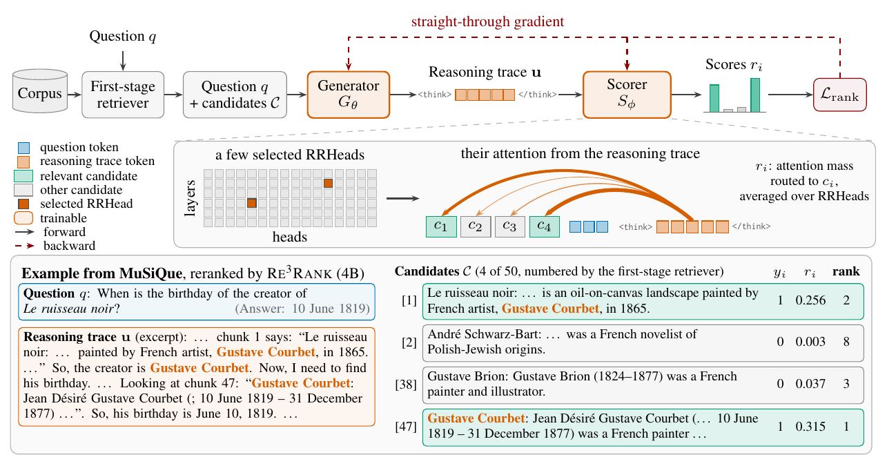
In online use, one request takes three steps:
- The generator reads "50 candidates + question" and writes a reasoning trace with greedy decoding, up to 1024 tokens.
- The scorer is a second model of the same size. It reads "50 candidates + question + this trace" and runs a single forward pass.
- Only two attention heads in the scorer, chosen in advance, are used. For each candidate, the attention every trace token sends to it is added up and averaged over all trace tokens to give its score, and candidates are sorted from high to low.
The scorer generates no text; the ranking is read directly from the attention of one forward pass. This differs from reasoning rerankers such as ReasonRank, which, after reasoning, still have to write the ranking out as a string of candidate IDs.
How each candidate's score is computed
is the set of selected attention heads, the positions of the trace tokens, the positions of candidate 's tokens, and the attention that position sends to position . Intuitively, it is "how much attention each word of the trace sends to this candidate, on average".
A small worked example (illustrative): the trace has only 2 tokens. In one head, token 1 sends 0.5 of its attention to the tokens of candidate [47] (summed), and token 2 sends 0.3. That head gives [47] a score of (0.5+0.3)/2=0.4. Another head gives 0.2, and averaging the two heads gives [47] a final score of 0.3.
Why only two heads
The 4B model has 1,152 attention heads, and most have nothing to do with finding evidence. Before training, the paper takes 800 labeled examples, lets the base model write a trace for each, and measures for every head the average attention that trace tokens send to relevant candidates, keeping the top two. For the 4B model these are (23,10) and (21,8), counted from 0, layer first and head second. Heads are picked once before training. During training, labels also mark which candidates are relevant in the ranking loss; online use needs no labels at all.
How it is trained: letting the ranking loss teach the generator
The scorer outputs continuous attention scores, so the ranking loss can be differentiated with respect to it directly. The generator is harder: it outputs sampled discrete tokens, and gradients cannot pass through them.
The paper uses a straight-through estimator. In the forward pass, the scorer still receives the embedding of the token the generator actually wrote, numerically unchanged. In the backward pass, it pretends that this position received a weighted average of all word embeddings, weighted by the probabilities the generator gave each word. The scorer's gradient can then flow through this weighted average and tell the generator which word probabilities at this position should go up and which should go down. The gradient is a biased approximation, but a single backward pass updates both the generator and the scorer. The scorer's word embedding table itself stays frozen. Hoot says

- Illustrative vectors: e(Courbet)=(1,0), e(Brion)=(0,1), e(Paris)=(−1,0). Suppose the direction that lowers the loss is (0.5, −0.2).
- How each word's probability should move is the dot product of this direction with its vector: Courbet 1×0.5+0×(−0.2)=0.5, raise; Brion 0×0.5+1×(−0.2)=−0.2, lower; Paris −1×0.5+0×(−0.2)=−0.5, lower.
- Where the bias comes from: the forward pass really read (1, 0), but the gradient is computed at the weighted average (0.5, 0.3); these are not the same point.
Illustrative: a 3-word vocabulary, 2-d word vectors, and made-up probabilities and gradient direction. The scorer's word-embedding table stays frozen. Source: paper §3.3 straight-through estimator: forward uses the generated token's embedding, backward takes gradients through the probability-weighted embedding; all numbers are illustrative.
The ranking loss has two parts. One is a contrastive cross-entropy: each relevant candidate is compared with all irrelevant candidates in the same pool and pushed to score higher. But this loss keeps widening gaps that are already in the right order. The other part targets the top-k boundary, with k set to 3 and 10. First, each relevant candidate gets a "soft rank": the score gap between every other candidate and it goes through a sigmoid, which approaches 1 as the gap grows, and these are summed plus 1 to give roughly where it ranks. Then "is the soft rank below k" is softened with a sigmoid as well and summed over relevant candidates, giving roughly how many relevant candidates are in the top k. The closer this count is to its attainable maximum, the smaller the loss, which amounts to optimizing Recall@k smoothly. By default the two parts are added at a 1:2 weight.
The training data is 38,000 English questions from 5 datasets including NarrativeQA and MuSiQue. For each question, Qwen3-Embedding-8B retrieves 50 candidates.
Results: who does the looking really matters
Evaluation uses 9 English datasets covering Wikipedia multi-hop QA, open-domain factoid QA, long-narrative QA, and long-conversation memory. All rerankers rerank the same 50 candidates.
| Method (average over 9 datasets) | R@3 | NDCG@10 |
|---|---|---|
| First-stage retrieval order | 62.09 | 70.27 |
| Qwen3-Reranker (4B) | 67.42 | 74.21 |
| ReasonRank (32B) | 72.31 | 78.34 |
| QRRanker (4B) | 73.39 | 79.12 |
| Re3Rank (0.6B) | 73.55 | 79.67 |
| Re3Rank (4B) | 76.70 | 82.23 |
The comparison to watch is QRRanker: both use a Qwen3-4B backbone and score by attention, but QRRanker looks with the question and Re3Rank looks with the trace. Their selected heads and training also differ. Re3Rank (4B) has higher NDCG@10 on all 9 datasets. ReasonRank also reasons first but then writes the ranking out as text, and at 32B it is still 4.39 R@3 points below Re3Rank (4B). The paper's explanation is that writing the judgment out as a string of IDs distorts it, and reading attention directly is more accurate.
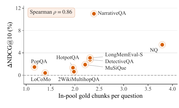
Where does the gain land? The more relevant candidates a question has, the larger the gain. PopQA and LoCoMo, with about one relevant candidate each, gain less than 1.5 points; NQ (Natural Questions, open-domain factoid QA), with nearly 4 relevant candidates on average, gains 5.45 points. The paper says this is consistent with traces helping most when relevant evidence spans several passages. The largest point is NarrativeQA, with an 11.00-point gain. It is an in-domain dataset: the training set also contains NarrativeQA questions, but they do not overlap with the evaluation questions.
How much does the trace itself contribute? The paper breaks it down with the same trained 4B scorer. Skipping the trace and looking with the question in the user turn gives 4.51 fewer R@3 points than the full trace.
Those 4.51 points come in two parts. Moving the question after <think> recovers 3.08 points, because that is where the scorer reads its queries during training. The trace content adds 1.43 points on top. A filler sentence with no content in that position still reaches 74.50 R@3, already above QRRanker. So within "who does the looking", position is the larger share, and the reasoning content adds a further step on top.
How much the generator and the scorer each contribute
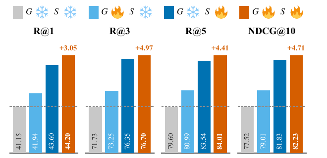
Without training, looking with traces written by the base model already gives 71.73 R@3, higher than the 69.16 from using the question. Training only the generator adds 1.52 R@3; training only the scorer adds 4.62; training both reaches 76.70, 0.35 more than training only the scorer. So most of the gain comes from training the scorer, and joint training adds a little on top.
On speed, when 50 questions are sent as one batch, the 0.6B version takes 0.26 s per question, slightly faster than QRRanker's 0.28 s, which means writing the trace costs little for a small model. The 4B and 8B versions take 0.81 and 0.93 s; my reading is that most of the cost is decoding the trace token by token.
Limitations as I see them
First, the candidate pool is always 50 candidates from the same retriever, and all candidates plus the trace must fit in the context at once. The average training input is already 9394 tokens; more candidates could exceed the context window, which the paper admits it has not tested.
Second, the trace is trained only by the ranking loss, so there is no guarantee that people can read it or that its content is correct. It is more like intermediate text built to steer attention, and should not be used as an interpretable rationale.
Third, latency is higher than pure scoring rerankers. The 4B version takes 0.81 s per question, while QRRanker needs only 0.28 s. The paper's appendix gives trade-offs: with a trace of only 64 tokens, the 4B and 8B versions already beat QRRanker; truncated to 256 tokens, the 4B version is only 0.26 R@3 below the full trace.
How a search team could try it
- Start without training: let an off-the-shelf base model write a trace, score your own candidates with its attention, and compare with scoring by the query. Include a control that places the query after <think>. The paper's appendix has such a control, with an untrained scorer and traces from the trained generator. There, the query after <think> gets 71.97, higher than the 67.95 from the full trace.
- Use a few hundred labeled examples to pick attention heads, the way the paper does: measure the average attention trace tokens send to relevant candidates and keep the top two.
- Train only the scorer first, since that is the biggest gain; add joint training with the straight-through estimator if you have capacity.
- Before launch, measure latency and truncate the trace to a length budget, choosing a point between quality and latency.
Verdict
Letting the scorer look from the position it was trained on, and then looking with a question-specific trace, together let a small model's reranking beat a much larger reasoning reranker.
| Aspect | Assessment |
|---|---|
| Problem importance | High. RAG reranking directly sets generation quality, and multi-hop questions are the hard part |
| Method novelty | Medium-high. Attention scoring is not new; turning "who looks" into a trainable reasoning trace is |
| Evidence | High. 9 datasets, 11 baselines, plus a breakdown that fixes the scorer and replaces the query text piece by piece |
| Engineering cost | Medium. One extra generation pass; the 4B version takes about 0.8 s per question |
| Worth trying | Yes, especially for multi-hop QA and long-conversation memory retrieval |
How did this read for you?
Hoot made a note. Thanks for the feedback.

One tap, no sign-in; tap again to undo. Only anonymous counts are kept, never who you are.
Discussion
Add experiment details, reproduction notes or a different take. Requires a GitHub sign-in.
Loading the discussion…