Contents · 11 sections
1What problem is it solving?2The whole pipeline first3Why let the three codes of one item know about each other?4The decoder: more capacity, gated attention5Five answers per history, and pushing down the group that was skipped6Post-training: beyond reward, get the order right7Serving: many items under one SID8Experiments: what the numbers say9Where I think it falls short10How a rec or search team could try it11Bottom lineSHARE

Generative retrieval generates SIDs, not items. Several items can share one SID, so which of them to pull from a SID is a separate decision. RedMall's authors are mostly from Xiaohongshu, and its online A/B tests run at the retrieval stage of industrial e-commerce recommendation and advertising; one of those tests isolates exactly this step. With the model unchanged, replacing "keep the top 40 items per SID by past sales performance" with "take all items under each SID, SID by SID, until the retrieval quota runs out" cuts the advertiser-value (ADVV) lift over the online baseline in the ads scenario from 2.24% to 1.1%, which is no longer significant. The model did not change, yet this lift went from significant to not significant; the only difference was how SIDs were turned into items. The model itself keeps the TIGER recipe of reading the history as SIDs and generating the next item's SID code by code, and strengthens it in four places: the input, the decoder, the training objectives and post-training. On the authors' industrial data these changes together lift HitRate@50 from 0.1416 to 0.1997. On public datasets its lead over the strongest baseline is thin, with two cells differing only in the fourth decimal place.
What problem is it solving?
RedMall gives every item a three-level SID, for example the paper's <s_a_8000><s_b_1000><s_c_76>. It comes from the item's text and image embeddings. Both are first post-trained on users' chronological interaction sequences with next-item prediction, so they carry behavioural signal about which items tend to be clicked one after another. For this sequence-aware multimodal representation step, the paper does not state which sequence model computes the next-item prediction or how the two embeddings are updated. They are then fused into one vector, which RQ-VAE quantizes level by level. Each level has a codebook, a set of learnable representative vectors called codewords, with 8,192, 1,024 and 128 codewords at the three levels. Each level picks the codeword nearest to the current vector, writes its index into the SID and passes the remaining difference to the next level. So the first level is a coarse group, and the second and third levels refine it. A user history is a sequence of such code triples, and the model generates the code triples of items the user may click or buy next, which are then mapped back to items.
Walk through one user (illustrative):
| When | What happened | What it means for training |
|---|---|---|
| Past month | Clicked 20 beauty items | This is the input history |
| Next | Clicked 5 more: a lipstick, a foundation, a makeup remover and others | Standard training uses only the first one as the answer |
| Same period | Was shown several perfumes, clicked none | Standard training ignores this |
The paper argues that existing methods miss four things here. The three codes are treated as a flat token sequence, although the second code refines the first, so this dependency is never modelled explicitly. NTP training supervises one next item per history, while retrieval has to return many items at once. Items that were shown but not clicked live only in exposure logs, which NTP cannot use. Reinforcement learning scores each candidate on its own and does not directly ask for the whole candidate list to be in the right order.
The whole pipeline first
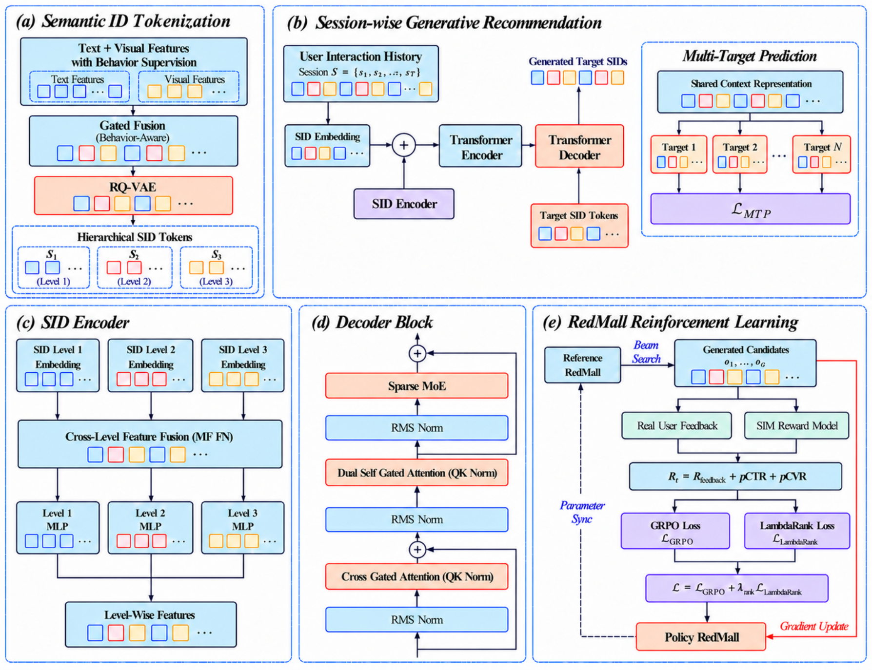
The pipeline, by what each stage produces:
| Stage | Input | Output |
|---|---|---|
| Item encoding | Text and image embeddings | A three-level SID per item |
| Encoder | SID tokens of the user history plus the SID encoder's added term | A user behaviour representation |
| Decoder | The user representation plus codes generated so far | The target SID, code by code; online beam width 50 |
| Supervised training | One history with 5 targets, plus a first-level code from unclicked exposures | Model weights |
| Post-training | A group of candidates and their rewards | The model fine-tuned with GRPO and LambdaRank |
| Serving | Generated SIDs | Up to 40 items per SID, chosen by past sales performance |
Encoder and decoder have four blocks each. The changes are spread across every stage and most come from prior work, the SID encoder being the main new piece, so the useful question is how much each one is worth. The rest of this piece follows the data flow.
Why let the three codes of one item know about each other?
In TIGER-style models every code in the history looks up its own embedding. Code 8000 gets the same vector whether it is followed by 1000 or 1003. The encoder's self-attention is fully visible, so the three codes can attend to each other, but the encoder has to learn from data which three tokens belong to the same item.
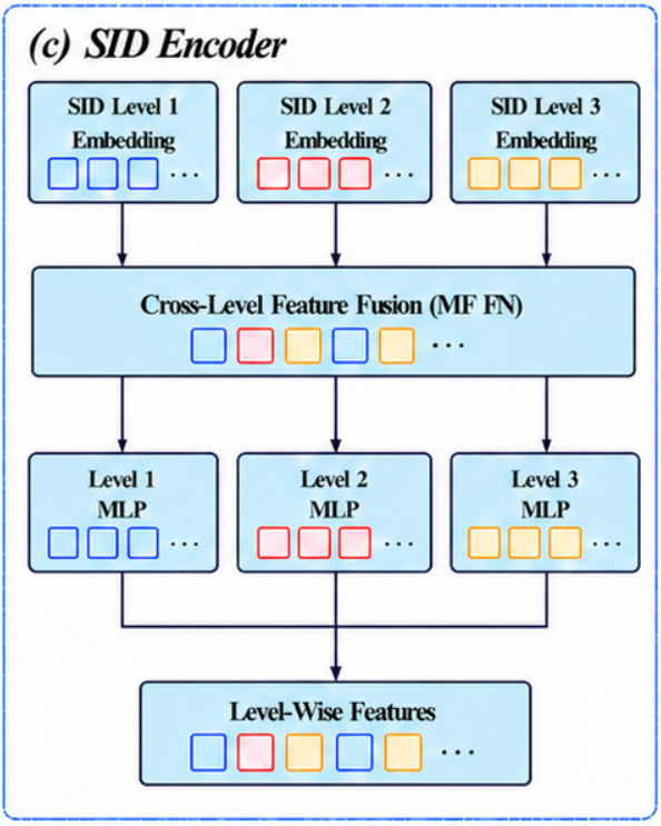
The SID encoder is simple. For each item in the history it looks up the vectors of its three codes, using the encoder's own embedding table. A small feed-forward network mixes the three into one fused representation , so each level's code can pass information to the other two. Three MLPs then map back to level-1, level-2 and level-3 features, and each is added to the input of the matching code token. The positional encoding is unchanged, which is where it differs from Tree-Transformer, another generative recommender that designs special positional encodings for the SID hierarchy.
An example (illustrative): two items have SIDs (8000, 1000, 76) and (8000, 1003, 12). Without the SID encoder, both occurrences of code 8000 enter the encoder as the same vector. With it, the first 8000 gets an added term computed from (8000, 1000, 76) and the second gets one computed from (8000, 1003, 12). The same coarse code already carries its item's finer codes before attention starts.
This module gives the largest single step in the industrial ablation: HitRate@50 goes from 0.1668 to 0.1832, 1.64 percentage points. It only changes the encoder input, and the authors call it plug-and-play.
The decoder: more capacity, gated attention
The decoder starts from TIGER's decoder, which the authors consider too small. They make two changes.
The feed-forward layers become a sparse MoE with 12 experts, of which 2 are active at inference. The model has about 0.5B parameters with about 0.1B active, so capacity grows while the compute per inference stays small. In the ablation this step adds 1.33 points, which hints that decoder capacity was one of the bottlenecks on the authors' data.
The second change is called Dual Gated Attention. Per the paper's Fig. 2(d), both the self-attention and the cross-attention of the decoder block become gated, following Qwen3's gated attention, with a gate that regulates how much of the attention output is kept. The paper counts one more change under this module: the causal mask over observed history items is replaced by bidirectional attention, so each history item sees both earlier and later interactions. On the encoder side the history is already fully visible; for Dual Gated Attention the paper does not say which decoder input or which attention's visibility the bidirectional history actually modifies. Gating and bidirectional attention together add only 0.28 points, the smallest of all modules.
Five answers per history, and pushing down the group that was skipped
Multi-target prediction (MTP) first. The last 5 items of each training sequence become targets and everything before them is the history shared by those 5 targets. The decoder runs once per target, each run still predicting that target's three codes one by one, and the five losses are summed:
Here is the shared history, is the -th code of the -th target item, and . The intuition: after 20 beauty items, both the lipstick and the makeup remover are good answers, and using only the first as the answer wastes supervision. The cost is also clear: decoder forward passes in training go up five times. This step moves HitRate@50 from 0.1416 to 0.1535.
Then the exposure-aware loss. For each target interaction, take items that were shown but not clicked within an exposure window of size 5 and use their most frequent first-level code as the negative target. Whether the window counts records or time, the paper writes only "window of size 5". Positives still have to generate all three codes; negatives only push down the first level:
is the selected negative first-level code and is the user history. The negative term is multiplied by a weight (the strength of negative feedback), added to the positive term, and divided by the number of positive and negative samples in the batch. By hand (illustrative): if the model gives the perfume code probability 0.30, this term is ; at 0.05 it is . Because only the first code is pushed down, the loss lowers a whole coarse group rather than one item. In the ablation this step goes from 0.1860 to 0.1948, 4.73% relative to the previous row.
Post-training: beyond reward, get the order right
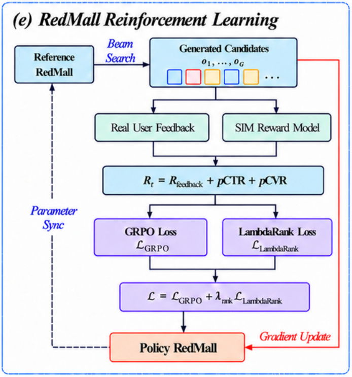
After supervised training the authors add a round of reinforcement learning. Each candidate SID's reward has two parts.
One part comes from real logs. Look at which items the user clicked in the following window (the paper's "future window", size 5, with no unit given), compare the candidate's three codes level by level with each clicked SID, and take the best match: 0 to 3 points, or 0 if there was no click. Levels are compared independently, so if the second code differs but the third matches, the third still scores a point.
The other part comes from a reward model. The online ranking model uses too many features to plug into training directly, so the authors use SIM as the reward model. The history enters as a SID sequence, the model outputs pCTR and pCVR for each candidate, and it is supervised by the online ranking model. The ranking model scores items, while the generated candidates are SIDs that may each cover several items. The paper does not say how SIM takes a candidate SID, or how item-level ranking supervision becomes SID-level pCTR and pCVR labels. The total is with .
A small group by hand (illustrative). The user later clicked (8000, 1000, 76). Candidate A is (8000, 1000, 12): two levels match, feedback 2, plus pCTR 0.04 and pCVR 0.01, total 2.05. Candidate C is (512, 7, 3): no level matches, so only pCTR 0.02 and pCVR 0.01, total 0.03. In this example each matched level is worth 1 point, far more than the pCTR and pCVR differences; when the window has no click, every candidate's feedback is 0 and only pCTR and pCVR separate them.
GRPO updates the policy with group-relative advantages; the group size is 32. That gives each candidate its own good-or-bad signal but does not directly require the model's probability order to match the reward order. LambdaRank fills that gap. With model score , for every pair where has the higher reward:
is the change in NDCG from swapping the two, so mis-ordered pairs that matter more for NDCG weigh more. Continuing the example (illustrative): if the model gives A a log-probability of −3.2 and C −2.5, the order is wrong and this pair's logistic term, before the weight, is ; with the order right and a gap of +0.7, it is about 0.40, and multiplying by the pair's NDCG weight gives its loss. The total loss is . In the ablation this step goes from 0.1948 to 0.1997, 0.49 points. GRPO and LambdaRank are added together as one row, so their shares cannot be separated. Hoot says

Order wrong (illustrative)
- reward
- A 2.05, C 0.03: A is better
- model log-probability
- A −3.2, C −2.5: the model prefers C
- score gap, A minus C
- −0.7
- ranking term
- about 1.10
The higher-reward A ranks lower, so this pair is penalised heavily.
Order right (illustrative)
- reward
- unchanged: A 2.05, C 0.03
- model log-probability
- A −2.5, C −3.2: the model prefers A
- score gap, A minus C
- +0.7
- ranking term
- about 0.40
A wider gap shrinks the term further, but never to 0.
Illustrative numbers, using candidates A and C from the text. On the left the model gives C the higher log-probability, against the reward order; on the right the two agree. The table shows the ranking term before the NDCG weight; the actual loss multiplies it by the pair's |ΔNDCG|.
Source
paper §3.2.4 Eq. (25)(26); numbers illustrativeServing: many items under one SID
Several items can share one SID. Taking every item under every generated SID fills the retrieval quota with a few SIDs. The authors score each item by two past-performance metrics: GPM (sales value per thousand impressions) and OPM (orders per thousand impressions).
Only the top 40 items per SID are kept. Illustrative: an item with GPM 120 and OPM 3 scores about 4.11; one with GPM 40 and OPM 6 scores about 3.36 and ranks lower. The logarithm flattens the score as sales grow, so doubling sales does not double the score.
The online ablation from the opening tests exactly this step. Without it, the advertiser-value lift is only 1.1% and not significant (p>0.05). The authors find that the share of retrieved items passing to downstream stages is then about half, mainly because duplicate filtering removes many of the retrieved items.
At inference, beam search runs with a KV cache, plus batched inference, multithreading and multiprocessing. Production runs on 24 NVIDIA L20 GPUs, serves about 120 million requests a day, and reaches up to 420 QPS per GPU.
Experiments: what the numbers say
The public datasets are Amazon Beauty, Toys, Food and MovieLens-1M, keeping each user's 20 most recent interactions and testing on the last one. The table shows NDCG@10 and Recall@10.
| Dataset | TIGER N@10 | Tree-Transformer N@10 | RedMall N@10 | TIGER R@10 | Tree-Transformer R@10 | RedMall R@10 |
|---|---|---|---|---|---|---|
| Beauty | 0.0395 | 0.0410 | 0.0418 | 0.0719 | 0.0723 | 0.0752 |
| Toys | 0.0418 | 0.0444 | 0.0468 | 0.0765 | 0.0766 | 0.0802 |
| Food | 0.0430 | 0.0460 | 0.0480 | 0.0806 | 0.0843 | 0.0877 |
| MovieLens-1M | 0.0912 | 0.1053 | 0.1059 | 0.1713 | 0.1929 | 0.1955 |
The gain over TIGER is clear, for example Recall@10 on MovieLens-1M from 0.1713 to 0.1955. Against Tree-Transformer RedMall leads on all 16 metrics, but some gaps are tiny: NDCG@5 on Toys is 0.0369 versus 0.0368, and on MovieLens-1M 0.0843 versus 0.0841. Table 1 reports no variance or run count, and gaps this small do not tell which model is stronger.
The industrial ablation (Table 3) says more about each component. Training uses 150 million users' clicked-item SID sequences from the previous month; evaluation uses 16,000 users, with each user's latest purchased item as the target.
| Configuration | HitRate@50 | Over baseline (points) |
|---|---|---|
| Baseline: NTP training | 0.1416 | 0 |
| Switch to MTP | 0.1535 | 1.19 |
| Add MoE | 0.1668 | 2.52 |
| Add SID encoder | 0.1832 | 4.16 |
| Add Dual Gated Attention | 0.1860 | 4.44 |
| Add exposure-aware loss | 0.1948 | 5.32 |
| Add RL | 0.1997 | 5.81 |
Two things to keep in mind. The Improvement column is the absolute HitRate difference, yet the text calls 1.19% a relative gain; the paper's Fig. 1(c) labels the total as 5.81 points, 41.03% relative. And each row is stacked on the previous one, with no leave-one-out comparison, so each step's gain depends on the order in which modules were added. Step by step, the SID encoder and the exposure-aware loss add 1.64 and 0.88 points, while gated attention and RL add only 0.28 and 0.49.
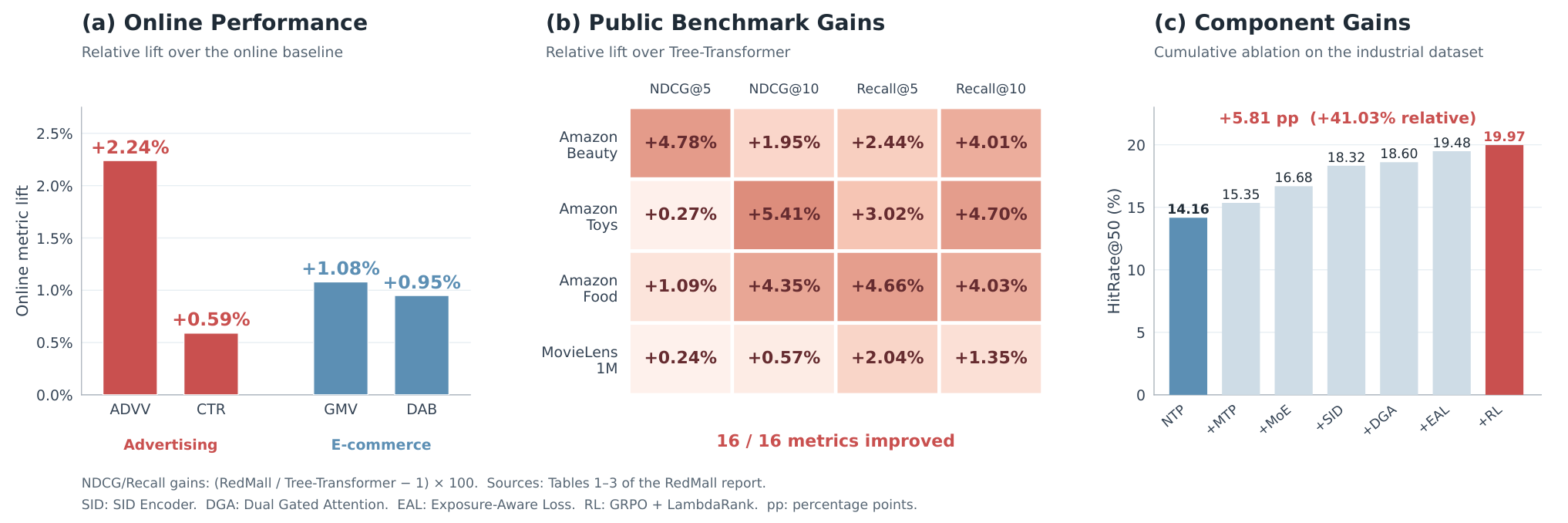
The online A/B tests all sit at the retrieval stage, with 10% versus 10% traffic for at least 7 days, and every metric has p below 0.05.
| Scenario | Metric | Change |
|---|---|---|
| E-commerce ads | CTR | +0.59% |
| E-commerce ads | ADVV | +2.24% |
| E-commerce ads | Cost | +0.56% |
| E-commerce recommendation | GMV | +1.08% |
| E-commerce recommendation | Daily active buyers (DAB) | +0.95% |
ADVV, advertiser value, is the main objective of the ads scenario. The paper gives only the name, with no formula in sight, so the 2.24% is best read as a direction rather than converted into revenue. In the ads scenario only items posted in the last 24 hours are candidates, a setting that favours SIDs: they are quantized from content-bearing item embeddings, so newly posted items get a SID right away.
Where I think it falls short
First, the public-dataset evidence is weak. The lead over Tree-Transformer is mostly between 1% and 5%, the two smallest cells are 0.27% and 0.24%, and there is no variance. The text says relative gains range from 0.14% to 8.16%, while Fig. 1(b), computed from the same table, shows 0.24% to 5.41%; the two do not match. Module ablations exist only on industrial data, and the four public datasets are user rating records, so the public table cannot tell us what the exposure-aware loss is worth.
Second, the ablation is cumulative. We can say the SID encoder contributes most in this order, not that removing it would cost 1.64 points; LambdaRank's own value is not visible either.
Third, exposure negatives only push down the first code. Items a shopper scrolled past may well share a coarse group with the item they finally clicked. If the chosen negative first-level code equals the positive's first-level code, the positive loss pulls that probability up while the negative loss pushes it down, and the two partly cancel. Window size and the most-frequent-code rule both affect how often this happens.
How a rec or search team could try it
Step one, for a team already running SID generative retrieval: add intra-SID item ranking, scoring items by past sales and keeping only the top few per SID. It does not touch the model and is the smallest change, and the paper's online ablation already shows how much it matters. Judge it by whether the share of retrieved items passing downstream goes up.
Step two: move training from one target to several, using the last few items of each sequence as answers. Only the data split and loss sum change, and decoder forward passes in training grow linearly with the number of targets. Compare offline HitRate and see whether the gain is close to the paper's 1.19 points.
Step three, where exposure logs exist: add exposure negatives and count how often the negative first-level code collides with the positive's. If collisions are common, filter those samples before judging the effect.
Step four: try the SID encoder and post-training. The SID encoder gave the largest single step on the authors' data and is cheap to add; post-training needs a reward model that takes SID sequences and is supervised by the online ranking model, and added only 0.49 points on the authors' data, so it goes last.
Bottom line
The key lesson: in production generative retrieval, the online gain also depends on which items are picked under each SID. This step does not change the model, yet with a different way of picking, the ads-scenario ADVV lift fell from 2.24% to 1.1% and was no longer significant.
| Dimension | Assessment |
|---|---|
| Problem importance | High. It gives one answer each for the input, supervision, post-training and item-selection problems of SID generative retrieval in e-commerce. |
| Novelty | Medium-low. Most parts come from prior work; the new pieces are the combination and the authors' own SID encoder. |
| Evidence | Medium. Industrial ablation and A/B tests in two scenarios are solid; the public-dataset lead is thin and ablations are cumulative only. |
| Engineering cost | Medium-high. MoE, five decoder passes per sample, a reward model and RL all add work; intra-SID ranking and the SID encoder are cheap. |
| Worth trying? | Yes, cheapest parts first. Intra-SID ranking and multi-target supervision can go first. |
| Fits | E-commerce recommendation and ad retrieval with large catalogues, many new items and an existing SID generative retriever. |
How did this read for you?
Hoot made a note. Thanks for the feedback.

One tap, no sign-in; tap again to undo. Only anonymous counts are kept, never who you are.
Related papersMore from Paper Daily
 Generative · 2026-11-02UGR: Unified Generative Ranking for Heterogeneous E-commerce RecommendationTaobao's generative ranking framework UGR has one generative model directly produce the screen the user finally sees. The roughly one thousand organic, ad and other-business candidates of a request go to the model together, and it generates the final list item by item, instead of each business ranking its own items and a blending stage stitching them together. That stitching step is the old probl…
 Generative · 2026-10-24UniRec: A Unified Expressive-Aligned Generative Recommendation Framework for E-commerceGenerative recommendation generates a product's semantic IDs layer by layer, and before the first layer it has seen no product-side information at all; this is its gap with discriminative ranking models. When a discriminative model scores a candidate it sees the product's category, shop and brand directly and crosses them with user features. UniRec has the model first generate the product's categ…
 Generative · 2026-03-05OxygenREC: An Instruction-Following Generative Framework for E-commerce RecommendationDeep dive: OxygenREC: An Instruction-Following Generative Framework for E-commerce Recommendation.
Discussion
Add experiment details, reproduction notes or a different take. Requires a GitHub sign-in.
Loading the discussion…