SHARE

In unified Transformer CTR models like OneTrans, adding positional encoding to the behavior sequence is the default, but the authors tried six positional encodings on Kuaishou's KuaiRand data (learned absolute positions, sinusoidal positions, RoPE, time-based RoPE and others), and none beat using no positional encoding at all (NoPE). A second observation: grouping past behaviors by how long ago they happened relative to this impression, letting behaviors in a group see each other while keeping order across groups, gives higher AUC than both per-behavior causal attention and fully bidirectional attention. Building on this, the Wuhan University and Tencent paper proposes TRIP (the authors' name for the whole method): each behavior encodes both its rank in the sequence and how long before this prediction it happened, and interacts in groups set by that time distance. On four public datasets it improves AUC over the strongest baseline by 1.47% relative on average, and by up to 4.45% on the Tencent ad dataset TAAC (a public Tencent ad-click sequence dataset).
Ranking teams should read it, because it answers a question rarely asked when copying language models: what is "position" in a CTR sequence? For the same history, change the impression time and every behavior's distance from now changes, while ranks and timestamps stay the same, something language-model positional encodings never had to handle. Every component has a matching ablation, and the positional encoding is validated separately on two more backbones. One caveat: all experiments are offline AUC on public datasets with no online results, and the group boundaries are fixed log intervals that do not adapt per user.
What problem is it actually solving?
Take an example (illustrative). A user recently clicked three items: a pair of shoes, a T-shirt and a pair of pants.
| Past behavior | Rank | Click time | Time before impression A (today noon) | Time before impression B (a week later) |
|---|---|---|---|---|
| Shoes | 3rd from last | yesterday noon | about 1 day | about 8 days |
| T-shirt | 2nd from last | today 11:00 | about 1 hour | about 7 days |
| Pants | last | today 11:59 | about 1 minute | about 7 days |
For impression A, the pants were one minute ago and nearly represent the current intent; the shoes were a day ago. For impression B a week later, all three are roughly "a week ago" and barely differ. Yet the rank (n-th from last) and the click timestamps are identical in both predictions. An encoding of rank alone cannot tell the two cases apart, nor can one of timestamps alone, because what decides a behavior's relevance is how long before this prediction it happened.
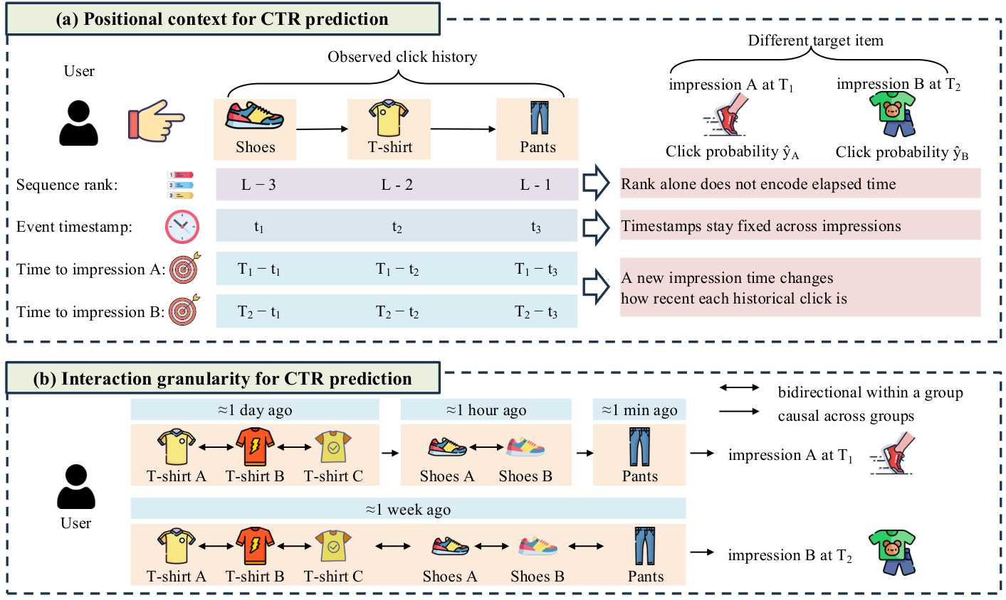
Interaction granularity follows the same logic. Two pairs of shoes viewed back to back within an hour reflect one interest, so letting them inform each other makes sense; causal attention lets only the later pair see the earlier one, splitting one interest into a sequence. Fully bidirectional attention goes the other way, mixing behaviors from a day ago and a minute ago and losing the direction in which interest evolves.
The pipeline
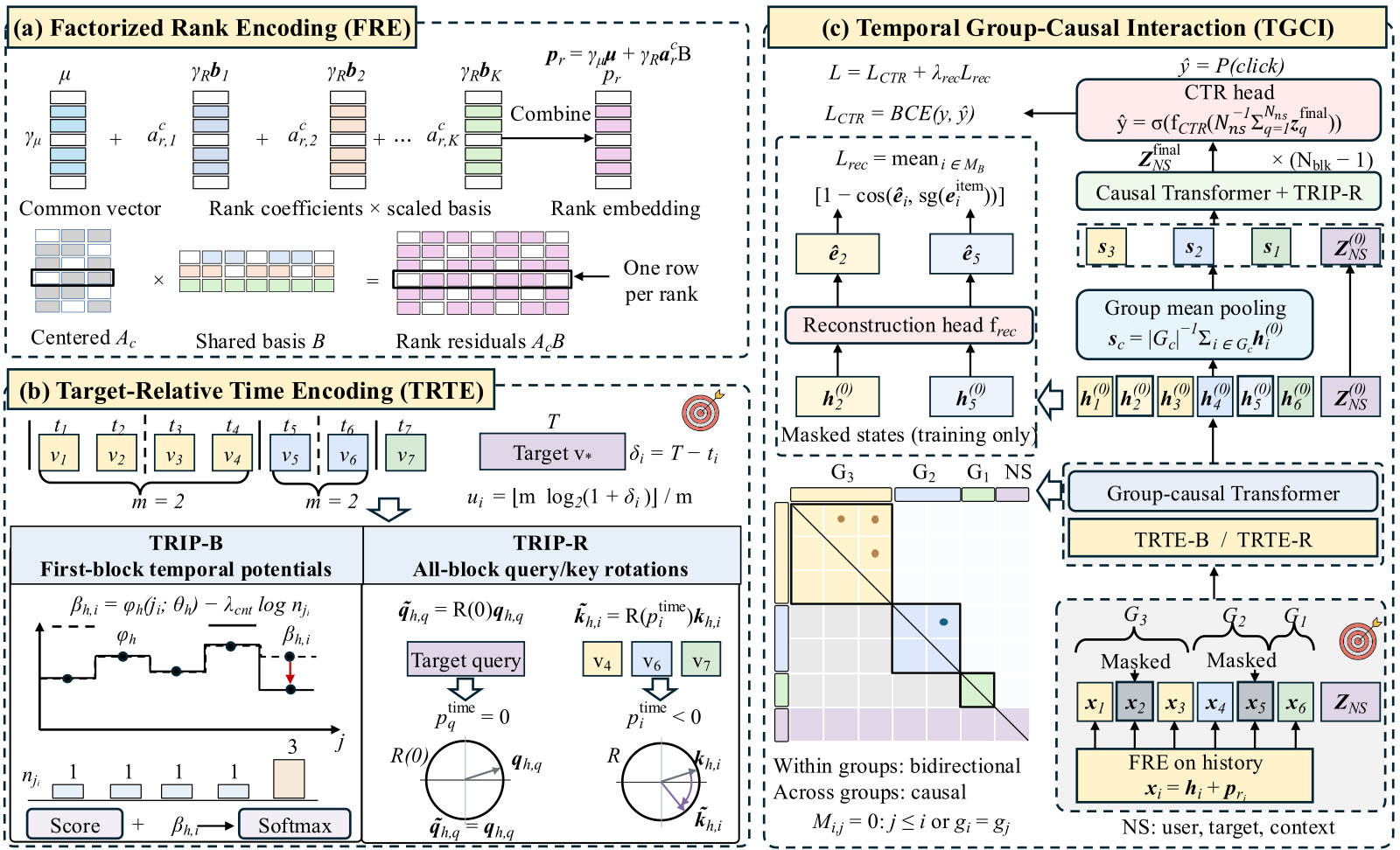
| Step | Input | What it does | Output |
|---|---|---|---|
| Rank encoding FRE | Each behavior's rank in the sequence | Represents each rank as a combination of a few shared basis vectors | A position vector added to the behavior token |
| Time encoding TRTE | Seconds between each behavior and this prediction | Converts to a log scale, then biases or rotates attention | Time preferences when prediction-side tokens read history (these comprise all non-sequential tokens constructed from user, candidate-item and contextual fields) |
| Group interaction TGCI | The same time distance | Groups by log interval, bidirectional within, causal across | One summary per group after the first layer |
| Later layers | Group summaries plus user, item and other non-sequential tokens | A standard causal Transformer | The CTR prediction |
The division of labor in one sentence: rank gives a behavior's context in the sequence, time distance gives its relevance to this prediction, and grouping decides which behaviors interact. The parts are explained below.
Why make the rank encoding low-rank?
The authors first observed that a learned absolute position embedding table in OneTrans, reconstructed with only a few PCA directions, loses almost nothing; 1 direction on TAAC and 4 on KuaiRand come close to the full table's AUC. So hundreds of position embeddings actually sit in a very low-dimensional space.
FRE (Factorized Rank Encoding, the authors' name) therefore splits the table in two: one common vector shared by all positions, plus each position's own K coefficients times K shared basis vectors. Parameters drop from L×D to D + L×K + K×D, where L is the sequence length and D the hidden size. On TaobaoAd, with length 300, hidden size 64 and K of 4, the full table needs 19,200 parameters and FRE only 1,520, about 12 times fewer. The coefficients are first centered across positions, so the common vector carries the shared "this is a history behavior" part and the coefficients carry only the differences between positions.
It is applied only to history tokens, not to non-sequential tokens. In the replacement experiment, FRE matches or beats the full position table on all four datasets.
How is time distance used?
TRTE (Target-Relative Time Encoding) first converts the seconds δ between each behavior and this prediction to a log scale:
m sets how many subdivisions each log interval gets. A log scale is fine near the present and coarse far away. Measured in seconds, 1 minute ago sits at about 5.9, 1 hour ago at about 11.8, 1 day ago at about 16.4, and 1 week ago at about 19.2. So about 6 steps separate a minute from an hour, but only about 3 separate a day from a week, which means recent time gaps are stretched and distant ones compressed.
With this scale, the paper offers two uses. TRIP-B learns a "time interval to bias" table per attention head and adds the bias to attention scores only in the first layer and only when prediction-side tokens read history, so different heads can learn different time preferences. TRIP-R works like RoPE: history behaviors sit on the negative time axis, prediction-side tokens at the origin, and query and key are rotated by the time coordinate in every layer. After compression, the model averages the behaviors' timestamps within each group and rounds the result to obtain the group summary's representative timestamp. Later layers use that timestamp to recompute the summary's target-relative time coordinates.
TRIP-B adds a density correction.
φ is the learned time preference, n is how many behaviors this sample has in that time interval, and λ is the correction strength. An example (illustrative): one interval holds 3 behaviors, another only 1, with equal content scores. Without correction, the first interval gets 3 shares of weight in total just because it has more behaviors. With λ of 0.5, each behavior's weight is multiplied by 3 to the power −0.5, about 0.58, for about 1.73 shares in total: the busier interval still leads, but no longer by a multiple. On all four datasets the best λ is nonzero; on KuaiRec AUC rises from 0.8488 without correction to 0.8510.
How do bidirectional-within, causal-across groups work?
TGCI (Temporal Group-Causal Interaction) groups by the same time distance: the group index is 1 plus log₂(1+δ) rounded down, capped at 32. So each group spans twice the time of the one before it. Once grouped, the attention mask has one rule: behavior i can see behavior j if and only if j comes before i, or both are in the same group.
With the opening example (illustrative): for impression A, the two pairs of shoes viewed an hour ago fall in one group and see each other; the pants from a minute ago are in a more recent group and can see the shoes, but the shoes cannot see the pants. For impression B a week later, these behaviors are all about a week old, mostly fall into one group, and all become mutually visible. Groups are recomputed for each prediction time, so the same history gets a different interaction structure for different impressions.
The input sequence places history tokens before prediction-side tokens. After the first layer, the model averages each group's behavior representations into one group summary. It then orders the summaries chronologically and uses them to replace the history tokens. Later layers process these summaries and the retained prediction-side states. Finally, all prediction-side states are mean-pooled and passed to the CTR head to produce the click probability. That shrinks the sequence for later layers from L behaviors to the number of non-empty groups. During training, some behaviors' item embeddings are randomly masked within each group, and the model reconstructs them from the other behaviors in the group as an auxiliary loss; this is turned off at inference.
Results
The experiments use four public datasets: Kuaishou short-video KuaiRec and KuaiRand, Tencent ads TAAC, and Taobao display ads TaobaoAd. They compare 11 models, including DCNv2, DIN, DIEN, RankMixer, and unified Transformer models such as OneTrans, HyFormer and MixFormer. All models share the same hardware, optimizer and training length, baselines keep timestamp features, and results average three random seeds.
| Model | KuaiRec AUC | KuaiRand AUC | TAAC AUC | TaobaoAd AUC |
|---|---|---|---|---|
| DIN | 0.8447 | 0.7705 | 0.6042 | 0.6235 |
| OneTrans | 0.8443 | 0.7694 | 0.6067 | 0.6276 |
| MixFormer | 0.8438 | 0.7754 | 0.6042 | 0.6265 |
| TRIP-B | 0.8512 | 0.7778 | 0.6337 | 0.6299 |
| TRIP-R | 0.8506 | 0.7731 | 0.6331 | 0.6292 |
TRIP-B has the highest AUC on all four datasets, with the clearest gain on TAAC. On KuaiRand its LogLoss is higher; the authors traced this to overestimated probabilities in one scenario with a very low positive rate, and fitting calibration parameters on validation data and then calibrating each model's outputs cuts the LogLoss gap between TRIP-B and MixFormer from 0.0300 to 0.0011, so the issue is calibration, not ranking ability.
Can the positional encoding stand alone? The authors remove group interaction and put only FRE plus the time encoding into three backbones, OneTrans, HyFormer and MixFormer, against eight positional encodings. In all 12 combinations at least one of the two versions has the top AUC; on TAAC, TRIP-R's encoding gives OneTrans a 4.20% relative gain. So this encoding does not depend on TRIP's other parts and transfers on its own.
Two ablation results best explain the design. Removing FRE or the time encoding drops TAAC AUC from 0.6337 to 0.6066 and 0.6073 respectively, so both are needed: rank and time distance carry different information. Replacing grouping with random groups or consecutive rank slices of the same sizes lowers AUC in every case, showing that the gain comes from grouping by distance to the prediction, not just from compression.
Compared with the version without group summaries, using group summaries reduces training time per step by 6.3% to 32.8% while AUC rises slightly. On TaobaoAd, TRIP-B takes 72.63 ms per step, on par with OneTrans's 73.78 ms and clearly faster than HyFormer's 147.23 ms.
Limitations as I see them
First, there is no online validation. All four datasets are public offline data, and outside TAAC the gains are in the third decimal place, KuaiRec going from 0.8449 to 0.8512; how much survives on industrial data is unclear.
Second, fixed log groups may not match real interest switches. The authors admit this: a user who switches from shoes to phones within ten minutes may have both behaviors fall in one log group. Whether they share a group depends on how long before the prediction each happened and where the fixed interval boundaries fall. Averaging within groups also blurs differences between individual behaviors.
Third, some hyperparameters are dataset-sensitive. FRE's K on TAAC lifts AUC from 0.6095 at 1 to 0.6340 at 10 and then declines; the time subdivision m is best finer on KuaiRand but best at 1 on TAAC and TaobaoAd, so it needs retuning per dataset.
How a ranking team could try it
- Start with the cheapest diagnosis: swap your sequence model's positional encoding for NoPE once. If results hold or improve, the current encoding is doing nothing.
- Add a log-scale bias for "seconds before this request", only on the attention where candidate tokens read history, with density correction. This leaves the architecture unchanged and is the easiest to ship and test.
- Replace the position table with a low-rank factorization and check that AUC holds with far fewer parameters.
- Try the group mask and group summaries last. They change the most but also save compute in later layers, which matters more for long sequences.
Verdict
The key takeaway: position in a CTR sequence should be defined with this prediction's time as the origin, not copied from language-model ranks.
| Dimension | Assessment |
|---|---|
| Problem importance | High. Unified Transformer rankers are spreading, and their positional encodings are almost all borrowed |
| Method novelty | Medium-high. No single part is complex, but taking the prediction time as the origin unifies positional encoding and interaction granularity |
| Evidence | Medium. Four datasets, 11 baselines, transfer across three backbones and careful ablations, but offline AUC only |
| Engineering cost | Low to medium. The time bias is nearly free; the group mask requires changing the attention implementation |
| Worth trying | Yes, especially the time bias and the NoPE diagnosis, which cost very little |
How did this read for you?
Hoot made a note. Thanks for the feedback.

One tap, no sign-in; tap again to undo. Only anonymous counts are kept, never who you are.
Discussion
Add experiment details, reproduction notes or a different take. Requires a GitHub sign-in.
Loading the discussion…