Contents · 7 sections
1The computation shared in one of Xiao Zhou's requests2Why pass a whole table instead of a single user vector?3AUC barely drops after the split4Where the model is split matters more than the RFM's own score5Two ways to shrink the table6The saved compute and the faster ranking path7Gains in two online experimentsSHARE

ByteDance's SepLRM paper shows that several ranking models on one platform can share a single encoding of a user's long history with almost no loss in quality, provided the models are split exactly where the candidate item first enters a computation with the user history.
On a large platform, many ranking models use the same user's history: e-commerce has pre-ranking and ranking, the mall has its own ranker, and advertising has another set. In recent years these models have all improved AUC and similar metrics by lengthening the behavior sequence and enlarging model capacity. The paper calls such models LRMs (large recommendation models, for example a ranking model that feeds a user's latest 10,000 behaviors into a Transformer).
The whole article uses one small scenario (illustrative). A user, Xiao Zhou, has 4 recent behaviors, in order: clicked running shoes, bought cat food, clicked running socks, viewed a litter box. The e-commerce ranker has to score a pair of running shoes, the mall ranker has to score a bag of cat food, and both models use this same history.
The difficulty is that cost and return are out of proportion. The scaling pattern the paper cites says LRM quality grows more and more slowly with compute, while training and serving cost grow roughly linearly or even faster. That cost is then multiplied by the number of models: a real sequence can reach 10,000 behaviors, the ranker encodes it once, and the mall ranker encodes it again. A typical model count in the authors' system is 30, so the same person's same history is encoded 30 times.
Existing approaches take one of two routes. The first makes each model cheaper on its own, for example by first selecting a short span of behaviors related to the candidate and modeling only that, or by switching to approximate attention that computes only some behavior pairs; each model still encodes the history separately. The second trains one large model first and then hands its computed results to the downstream rankers. Such a shared large model is called an RFM (recommendation foundation model).
The problem with the second route is that what gets handed down is too coarse. Among existing RFMs, LLaTTE hands down a compressed user embedding: Xiao Zhou's running interest and cat interest are squeezed into one vector, and the running shoes and the cat food receive exactly the same thing when they are scored. Rec-Distill hands down the large model's score for each candidate (logits), which the downstream model can only use as a learning target; if the downstream model wants to look up which of Xiao Zhou's behaviors relate to its own candidate, that score has nothing to look up.
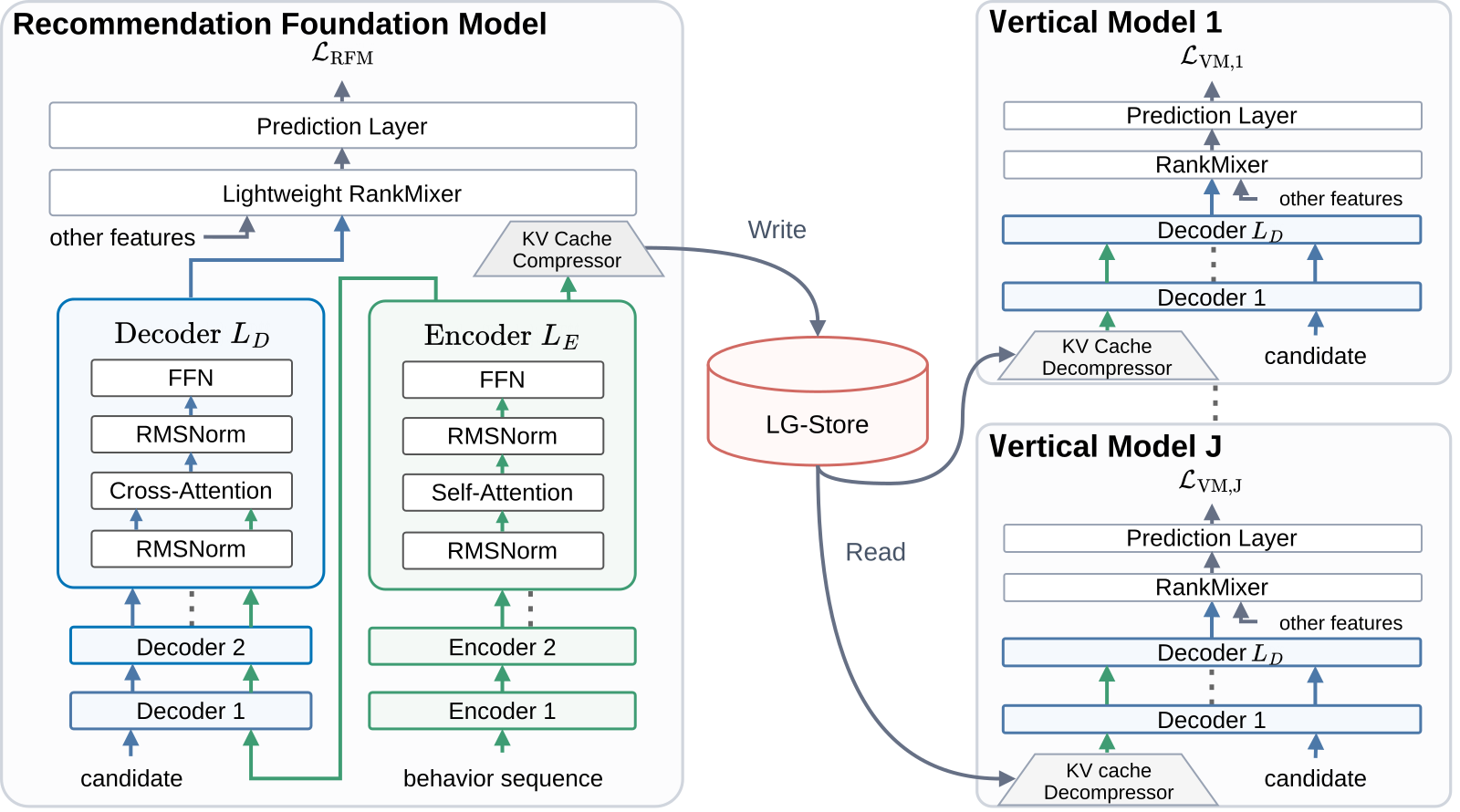
SepLRM changes what the RFM hands down. One RFM is dedicated to encoding the user's long history and exports the encoded state of every behavior as a table, one row per behavior, as the next section explains. Each business model (the paper calls it a vertical model, VM (a business-specific downstream model), for example the mall ranker above) uses its own candidate to draw information from this table according to relevance. On offline Douyin e-commerce data, the VM after this split reaches an AUC of 0.85010, exactly the same as an end-to-end model of the same scale trained as one piece without the split.
The computation shared in one of Xiao Zhou's requests
The table below walks through SepLRM's four steps with Xiao Zhou's example. The first two steps run once; the last two run once for each VM.
| Step | Who does it | Input | Operation | Output |
|---|---|---|---|---|
| 1. Encode history | The RFM's encoder | Xiao Zhou's 4 behaviors | Each behavior runs self-attention over the behaviors before it, stacked over several layers, with no candidate involved at any point | 4 state vectors, one per behavior |
| 2. Compress and store | RFM | 4 state vectors | Dimension reduction, quantization | KV cache (a table with one row per behavior, name explained below), written to a dedicated storage system |
| 3. Draw information | Each VM's decoder | KV cache, the VM's own candidate and request context | Decompress the cache, turn the candidate features into query vectors, use cross-attention to weight every row of the cache and take the weighted sum | The user interest representation for this candidate |
| 4. Score | Each VM | Interest representation, non-sequence features such as age | Combine the interest representation with the other features (feature interaction), then a prediction head outputs the score | This candidate's predicted score |
In training, the RFM and the VMs are trained separately on their own data and objectives: the RFM writes its computed cache to storage, and the VM reads it back as input during training. The RFM also keeps its own decoder, a light feature-interaction module and a prediction head, so that the RFM has a prediction task of its own and the encoder receives a training signal. When a request arrives online, the system prepares the cache at the same time as retrieval and pre-ranking run; it can run steps 1 and 2 on the spot or read a cache that is already stored. Only after the candidates chosen by retrieval and pre-ranking enter downstream ranking does each VM run steps 3 and 4.
The KV cache is just a table in which each of the user's behaviors takes one row. Xiao Zhou's table looks like this (illustrative):
Row 1  clicked running shoes   [1, 0]
Row 2  bought cat food         [0, 1]
Row 3  clicked running socks   [1, 0]
Row 4  viewed litter box       [0, 1]
A real row has 512 dimensions by default and already carries information from the behaviors before it. Here only 2 dimensions are written so the arithmetic is easy: treat dimension 1 as running-related and dimension 2 as cat-related. In cross-attention this table supplies the keys and values, which is why the paper calls it a KV cache. Every layer of each VM's decoder multiplies the same table by its own learned matrices to get the keys and values that layer needs, so the table only has to be stored once.
Why pass a whole table instead of a single user vector?
A single user vector is far cheaper than a table with 10,000 rows, so it is natural to want one more step of compression: squeeze the whole table into one user vector and pass that down. Illustration: averaging Xiao Zhou's 4 rows gives [0.5, 0.5], where averaging stands in for any method that compresses a whole history into one fixed vector. The running shoes and the cat food both receive [0.5, 0.5]; the running interest and the cat interest are already mixed together, and this part of the downstream model's input is identical for the two candidates. Hoot says

Compress to one vector
- Source
- compressed user vector
- Queries
- own short sequence
- User A
- (0.5, 0.5, 0)
- User B
- (0.5, 0.5, 0)
- Run/cook
- can be reweighted
- Off-road
- A, B look alike
From this vector alone, A and B give identical input, so any downstream model treats them the same.
Keep per-behavior states
- Source
- final encoder states
- Queries
- full history
- User A
- off-road 0.6
- User B
- off-road 0
- Run/cook
- picked per behavior
- Off-road
- A, B differ
Illustrative weights: the off-road query gives the first behavior 0.7 and the others 0.1 each. A = 0.7×1 + 0.1×(−1) = 0.6; B's off-road values are all 0, so it reads 0.
Illustrative: each behavior is three numbers (running, cookware, off-road), and averaging stands in for compression. User A's four behaviors are an off-road shoe (1, 0, 1), a road shoe (1, 0, −1), and two pans (0, 1, 0). User B's two shoes are both a plain model (1, 0, 0), with the same two pans. The source and query target in the left column follow LLaTTE; the averaging is only illustrative. Downstream models can still reweight the running and cookware dimensions using the candidate; what cannot return is the per-behavior difference averaged away. In training, the RFM and VMs are optimized independently: the RFM writes the cache late in its training, and each VM reads it in its corresponding later stage, optimizing only its own decoder, feature interaction, and prediction heads. Online, the cache is either computed by calling the RFM when a request arrives or prefetched from LG-Store.
Source
paper §1 (the KV cache keeps finer behavioral information than logits or aggregated user embeddings); §3.2.2 Eq. 9 and §3.3 Eq. 12 (producing and reading the cache); §3.1, §3.4.1 (independent optimization, late-stage writes and reads); §4.2 (precomputation and prefetching); §5.2 (LLaTTE). The shoe and pan vectors and the attention weights are illustrativeKeeping the whole table lets the VM have each candidate compute its own weights, which means different candidates can draw different content. Cross-attention computes weights from how similar the query is to each row, and the weights sum to 1. Illustration: the running-shoe query gives the 4 rows weights of 0.4, 0.1, 0.4 and 0.1, and the weighted sum is [0.8, 0.2]. The cat-food query gives the 4 rows weights of 0.1, 0.4, 0.1 and 0.4, and the weighted sum is [0.2, 0.8]. So the same table does not need to be re-encoded: switching candidates only means recomputing one set of weights, and the two candidates draw different content.
This table can be shared by several models only if it does not depend on the candidate. In step 1, neither the running shoes nor the cat food took part in the computation, so the ranker and the mall ranker can share the table, each bringing its own candidate to draw information. The cross-attention a VM runs is the same kind of computation as inside an end-to-end model, so the paper expects no loss in quality after the split.
AUC barely drops after the split
To know how much quality the split costs, two reference models are needed. NoSeq is the E2E LRM below with its long-sequence part removed, representing the level reached with no long history at all. The E2E LRM has the same sequence structure and capacity as SepLRM but is trained end to end, representing the level reached without the split. TR (transfer rate) measures how much of the long-sequence gain the VM keeps, computed as (VM AUC − NoSeq AUC) divided by (E2E AUC − NoSeq AUC).
Illustration: NoSeq is 0.80, E2E is 0.84 and the VM is 0.83. The long sequence could bring 0.04, the VM got 0.03, so TR is 75%.
The table below shows results on three datasets: Douyin e-commerce and Hongguo short dramas are ByteDance industrial data, and KuaiRand-27K is public. The SepLRM column reports the downstream VM's AUC. The RFM has a 6-layer encoder plus a 6-layer decoder, the VM is a 6-layer decoder, and the other methods use the same layer counts and training configuration.
| Dataset (max sequence length) | NoSeq | LLaTTE | E2E LRM | SepLRM |
|---|---|---|---|---|
| Douyin e-commerce (10,000) | 0.84131 | 0.84909 | 0.85010 | 0.85010 |
| Hongguo short dramas (5,000) | 0.84162 | 0.84740 | 0.84798 | 0.84798 |
| KuaiRand-27K (5,000) | 0.64640 | 0.68142 | 0.68307 | 0.68308 |
Across the three datasets, SepLRM differs from the unsplit E2E LRM by at most 0.00001. This shows that when the cache has no compression loss, splitting the model into an RFM and VMs loses almost no AUC, and TR is about 100%.
On Douyin e-commerce LLaTTE is 0.00101 below SepLRM. The paper treats an absolute gain of 0.0001 as already meaningful for the business, so 0.00101 is about ten times that size. The authors' explanation is that LLaTTE compresses the long history into a fixed user embedding, so when the downstream model runs attention it can only search its own short behavior sequence; the long history enters downstream only as that one vector, and its details never reach the downstream model.
Where the model is split matters more than the RFM's own score
The results above rest on a structural premise: the RFM has a clean boundary between its encoder and decoder. The encoder processes only behaviors throughout, and every decoder layer draws from the same final encoder state, so passing only that final state is enough. The other two RFM structures the paper compares, encoder-only and decoder-only, have no such boundary: the candidate interacts with that layer's behavior representation at every layer.
Illustration: the model has 3 layers. When it is split between encoder and decoder, all 3 decoder layers draw from the same 4-row table, so passing 1 table is enough. A model in which the candidate interacts layer by layer needs the behavior representations of layers 1, 2 and 3 separately, that is, 3 tables; if only the last one is passed, the VM cannot reproduce the interactions in the first two layers.
The authors also verified that, with these two RFM structures, passing the behavior-side keys and values of every layer to the VM restores TR to 100%, at the cost that what must be passed grows from one table to one table per layer, which greatly increases storage and communication. The table below fixes the VM and changes only the RFM's structure and its feature-interaction module. The feature-interaction module combines the candidate's interest representation with features such as age into higher-order combinations, and "none" in the table means the module is removed.
| RFM structure | RFM feature-interaction parameters | RFM's own AUC | VM AUC | TR |
|---|---|---|---|---|
| encoder + decoder | 4 billion | 0.85010 | 0.85010 | 100% |
| encoder + decoder | 700 million | 0.84883 | 0.85010 | 100% |
| encoder + decoder | none | 0.83213 | 0.84969 | 95% |
| encoder-only | 4 billion | 0.85011 | 0.84918 | 89% |
| decoder-only | 4 billion | 0.85017 | 0.84926 | 90% |
The RFMs in rows 1, 4 and 5 have almost the same AUC of their own, 0.85010, 0.85011 and 0.85017, yet their TR is 100%, 89% and 90%. This shows that RFMs with nearly identical AUC of their own can export caches whose downstream TR differs by more than ten percentage points.
Whether a shared cache is good depends on how much gain the downstream VM gets from it; the RFM's own AUC does not tell you that.
The first 3 rows answer a different question: does the RFM need strong feature interaction? Shrinking this module from 4 billion parameters to 700 million and then removing it entirely drops the RFM's own AUC from 0.85010 to 0.83213, while TR stays at 100%, 100% and 95%. This shows that feature interaction mainly affects the RFM's own scores and barely affects the exported cache; the cache's quality comes mainly from sequence encoding, so the RFM's parameter budget should go to the encoder first.
Two ways to shrink the table
For a history of 10,000 behaviors, with the default 512 dimensions per row and 16 bits per number (BF16), a rough estimate at this upper bound puts one sample's cache at about 10 MB. The paper compresses in two directions: make each sample's cache smaller, or remove behaviors stored repeatedly across the many samples of one user.
Compressing a single cache again comes in two kinds, and the first four rows of the table below each try two settings. Quantization reduces the bits per number: INT8 uses 8 bits and INT4 uses 4, so storage falls to one half and one quarter of the default. Dimension reduction reduces the numbers per row, from 512 dimensions to 256 or 128, so storage likewise falls to one half and one quarter.
| Compression | Setting | Storage relative to default | VM AUC | TR |
|---|---|---|---|---|
| Quantization | INT8 | 50% | 0.85013 | 100% |
| Quantization | INT4 | 25% | 0.85001 | 99% |
| Dimension reduction | 256 dims | 50% | 0.84974 | 96% |
| Dimension reduction | 128 dims | 25% | 0.84952 | 93% |
| Switch to user-level cache | user-level | 1.3% | 0.84936 | 92% |
At the same 25% of storage, INT4 keeps 99% of TR while 128 dimensions keeps only 93%. This shows that when storage is tight, cutting the bits per number pays off better than cutting the dimensions per row.
The user-level cache in the last row removes repetition across samples. The default sample-level cache stores a whole table for every sample, so a user's many samples repeatedly store many identical behaviors. Illustration: Xiao Zhou makes 3 requests, with histories of 2, 3 and 4 behaviors at the time; sample level stores 9 rows in total, while user level stores 2 rows the first time and then appends 1 new behavior each of the next two times, 4 rows in total.
The user-level cache is stored by user id, and besides the behavior state each row records the behavior time and the time of the request that wrote it. Xiao Zhou's record looks like this (illustrative), one row per pair of parentheses: the behavior state, when the behavior happened, and which request wrote it into the cache.
Xiao Zhou → [
  (state of shoe click,      behavior 09:50, request 10:00),
  (state of cat-food buy,    behavior 10:20, request 11:00),
  (state of sock click,      behavior 10:40, request 11:00),
  (state of litter-box view, behavior 11:30, request 12:00),
]
These timestamps prevent training from using future information. Training shuffles the sample order, so when an early sample is processed, a later request may already have written states it computed into the cache; the paper filters out that content as well. Illustration: a sample whose request time is 10:50 reads Xiao Zhou's cache. The behavior-time filter removes the 11:30 litter box, the request-time filter then removes the three rows written at 11:00 and 12:00, and only the running shoes remain.
Cat food and running socks clearly happened before 10:50 yet cannot be read; this is the loss of the user-level cache. The VM adds a light encoder dedicated to these recent behaviors that cannot yet be read, and the VM's decoder uses these few recent behaviors together with the history in the cache to fill the gap.
The last row of the table above shows that the user-level cache cuts storage to 1.3% of the default while keeping 92% of TR. This shows that most of the long-sequence gain can be kept with very little storage, at the cost of 8 percentage points of TR relative to the default, so the choice of granularity depends on the storage budget and on whether the cache is to be reused across stages and scenarios (see the next paragraph).
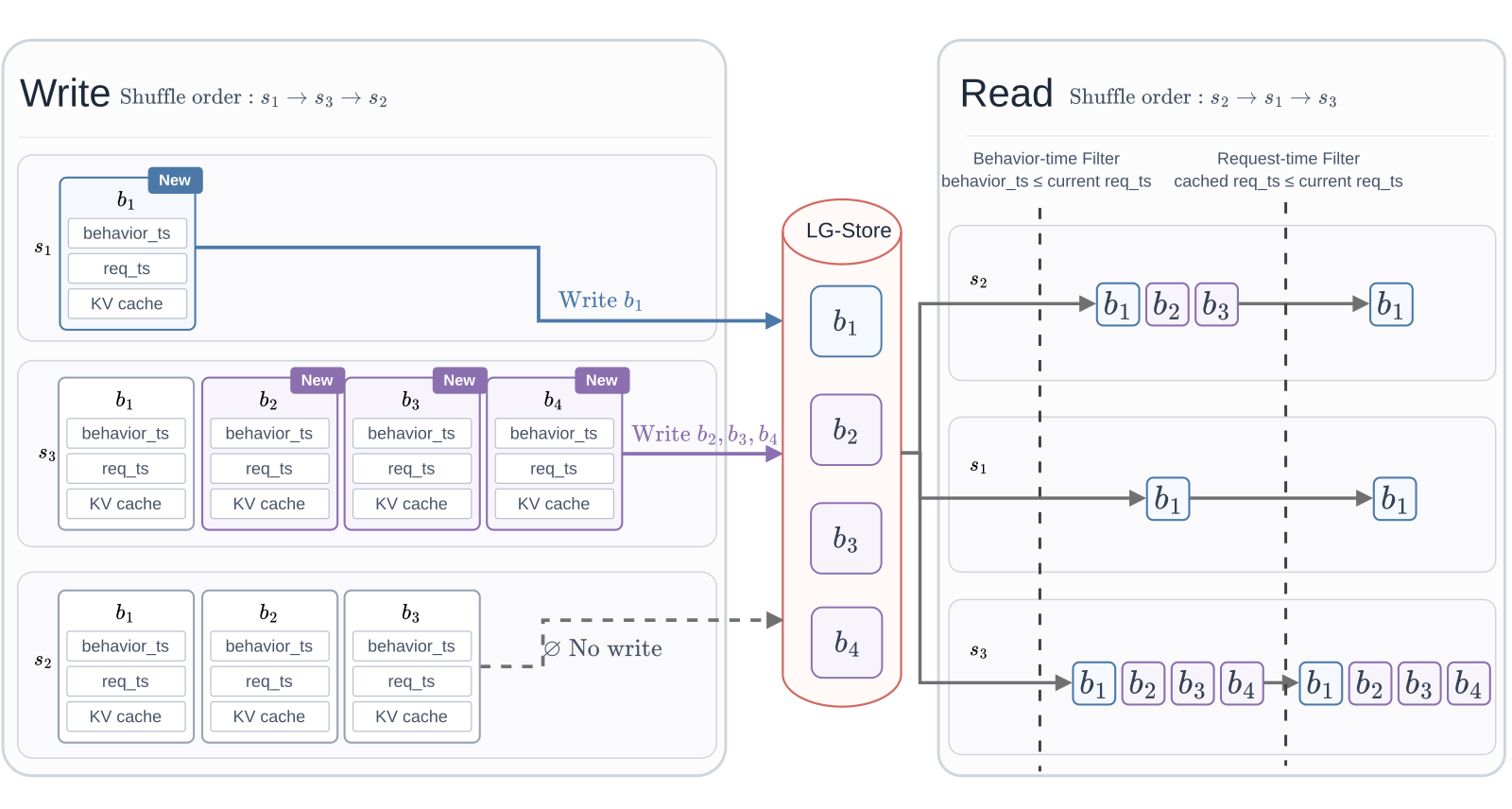
The user-level cache also enables reuse across models. A sample-level cache is looked up by sample id, and the training samples of pre-ranking and ranking are two separate data streams whose ids do not match; a user-level cache is looked up by user id, so both sides find the same cache for Xiao Zhou. The authors took the user-level cache of an RFM trained on e-commerce ranking data and gave it to two other models: relative to base models without the cache, e-commerce pre-ranking AUC rose by 70×10⁻⁴ and mall ranking AUC by 10×10⁻⁴.
E-commerce pre-ranking has many candidates and a tight latency budget, so it often cannot afford full long-sequence modeling. A pre-ranking AUC gain of 70×10⁻⁴ shows that pre-ranking can use the long history by adding only a light decoder; the mall's feature distribution and training objective both differ from e-commerce ranking, and the same cache still helps there.
These caches live in LG-Store, a distributed storage system ByteDance built for large-scale caches. Under the same throughput, durability and tail-latency requirements, LG-Store lowers average batch read latency by 64% and costs 43.5% as much as a conventional disaggregated KV storage system. This shows that the new cost of storing and reading caches can be kept down with dedicated storage.
The saved compute and the faster ranking path
Almost all of the cost of a long sequence is in the encoder. Illustration: self-attention over 10,000 behaviors, ignoring constants and layer counts, is about 100 million pairwise computations. The decoder's queries come from the candidate and the request context and are few; take 10 here, each computed against 10,000 rows, about 100,000 computations, a 1,000-fold difference.
Count one decoder pass as 1 unit and one encoder pass as 1,000 units (illustrative). Thirty end-to-end models cost 30×1001, or 30,030 units. SepLRM is 1 encoder plus 31 decoders, the extra decoder belonging to the RFM, for 1,031 units plus the cache overhead. This shows that the more models there are, the more is saved: the saving is roughly (number of models − 1) encoder passes, so 30 models save 29.
The ranking path gets faster through parallelism. The paper counts the end-to-end model's latency this way: retrieval and pre-ranking first, then sequence encoding, then prediction, with the three times added in sequence. SepLRM starts preparing the cache as soon as the request arrives, at the same time as retrieval and pre-ranking, and as long as cache preparation is no slower than retrieval plus pre-ranking, the sequence-encoding time drops off the critical path. SepLRM prepares the cache in one of two ways: call the RFM on the spot to produce a fresh cache, or read an existing cache from LG-Store, whose freshness depends on how often it is updated.
Illustration: retrieval plus pre-ranking takes 60 ms, sequence encoding 40 ms, downstream scoring 30 ms. The serial total is 130 ms; in parallel it is max(60, 40) + 30, or 90 ms, saving exactly the 40 ms of encoding. If cache preparation takes 80 ms, the total becomes 110 ms and only 20 ms is saved. This shows that as long as cache preparation takes no longer than retrieval plus pre-ranking, the ranking path saves the whole encoding step.
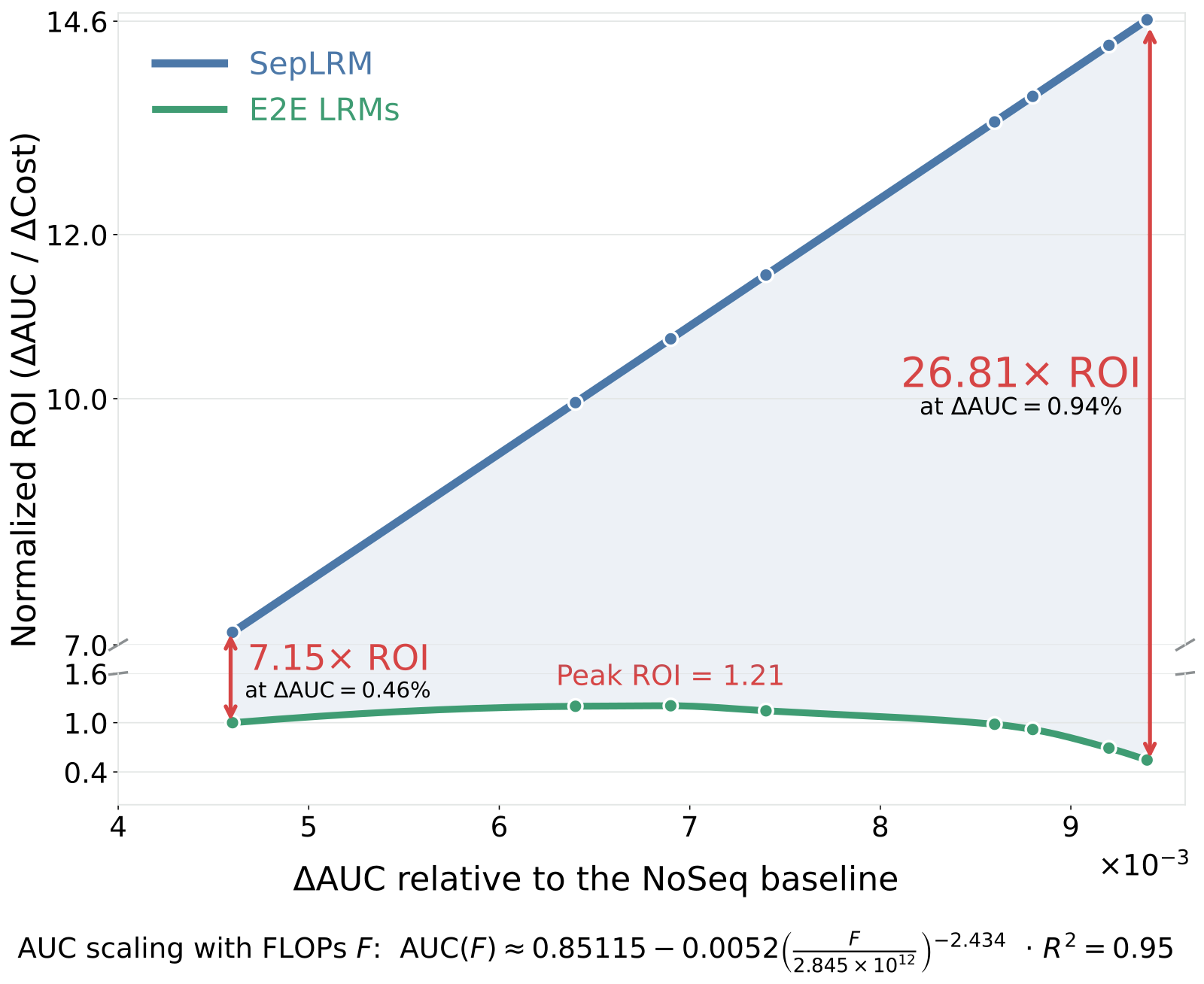
The authors ran the experiment in the figure above on e-commerce data to see how return on investment changes as the model grows: sequence length goes from 200 to 10,000, and the encoder and decoder each go from 2 to 8 layers. ROI is the offline AUC gain over NoSeq divided by the cost increase, with cost computed from accelerator hours and unit price. SepLRM also pays for 30 days of cache storage, so the cache overhead is already in this calculation. A typical model count in the authors' system is 30, so the calculation assumes 30 models.
The end-to-end model's ROI first rises and then falls, while SepLRM's ROI keeps rising, and the ratio of SepLRM's ROI to the end-to-end model's grows from 7.15 to 26.81 times. This shows that with 30 models sharing one RFM, the longer the sequence, the more sharing is worth; once the end-to-end model is scaled past a certain size, the AUC gain bought by each unit of cost actually falls.
Gains in two online experiments
In both online A/B experiments, the control group is the existing online model each business has optimized for a long time, and the treatment group switches to SepLRM.
The first experiment ran in advertising on GIP (General Information Platform, ByteDance's general information platform, which includes Hongguo, Toutiao and Fanqie Novel). The model used 10,000-behavior sequences with a 4-layer encoder plus a 4-layer decoder; the treatment group received 20% of online traffic for 9 days. The advertiser score (ADSS) rose 1.961% and advertiser value (ADVV) rose 2.107%. Both metrics rose on all three apps, Hongguo, Toutiao and Fanqie Novel, by between 1.311% and 2.492%. This shows the gain does not depend on any single app.
Douyin e-commerce used 5,000-behavior sequences with a 6-layer encoder plus a 6-layer decoder, with 30% of traffic for 14 days. In short-video e-commerce, orders per user rose 4.6306% and GMV per user rose 4.8077%; in live-stream e-commerce they rose 0.3673% and 0.3524%. This shows the same approach gains very differently across content formats: the short-video GMV gain is more than ten times the live-stream one.
These two A/B tests answer "how much more does switching to SepLRM earn"; because the control group is the online model, they do not by themselves show how much the split saves compared with not splitting. To answer that, the authors computed the ROI of E2E LRM and SepLRM at the same deployment scale, using the same method as the previous section. On GIP advertising E2E LRM is 26 and SepLRM is 224, 8.62 times; on Douyin e-commerce they are 319 and 835, 2.62 times. This shows that at both real deployment scales, the split approach gets a higher return on investment.
Back to Xiao Zhou's example, the paper's approach comes down to one thing: that 4-row table is computed once, and the ranker and the mall ranker each bring their own candidate to draw information from it. If you move this into your own system, the way to judge whether the split is right is to look first at the downstream VM's AUC and TR; how much the RFM's own AUC rose does not answer that question.
How did this read for you?
Hoot made a note. Thanks for the feedback.

One tap, no sign-in; tap again to undo. Only anonymous counts are kept, never who you are.
Discussion
Add experiment details, reproduction notes or a different take. Requires a GitHub sign-in.
Loading the discussion…