SHARE

Customer-facing LLM agents are usually bound by dozens of behavioral rules, such as "compensate only if the passenger bought travel insurance". Every turn, the agent must first decide which rules apply to the current situation and then put them in the prompt. Parlant's engine used to ask an LLM "is this policy relevant now?" once per policy per turn; with 36 policies that is 36 LLM calls and about 69,000 prompt tokens per turn. The Parlant team's Signals and Queries (S&Q) replaces this step with small classifiers trained offline. For each policy, an LLM writes, offline, 10 user messages that should trigger it and 10 user messages that look similar but belong to a neighbouring policy. These are embedded, and a separate logistic regression is fitted for that policy. At run time each turn needs one embedding call and 36 dot products, 37 microseconds of CPU, and the authors estimate per-turn cost is roughly 100,000 times lower than asking an LLM per policy. On 254 conversation states from τ²-bench airline customer service, taking the LLM judge as ground truth, S&Q reaches 32% precision at ≥90% recall with Gemini embeddings and 34% with OpenAI embeddings, only 1 to 3 points above a plain cosine threshold. Switching to exemplars mined from real conversations lifts precision to 43.5% and 41.6%. The paper's real value is not its default numbers but that it pins the bottleneck on where the exemplars come from.
1. The problem: missing a rule is an error, an extra rule is just waste
Stuffing every rule into the prompt each turn does not work. Content in the middle of a long context tends to be ignored, attention per instruction gets diluted, adherence drops as instructions pile up, and token cost grows linearly with the number of rules. So the relevant rules have to be filtered first.
The cost of filtering is asymmetric. Miss the cancellation policy and the agent may do something it should have refused; include an irrelevant rule and you spend a few hundred extra tokens. S&Q therefore first guarantees at least 90% recall per rule and only then improves precision. It is a pre-filter: a rule filtered out can never be recovered later, while the surviving rules are read again by the agent's own LLM, which can ignore the irrelevant ones.
The cheapest option is to compare the conversation directly against the rule text by embedding similarity, but it works poorly. Conversations are informal user messages, rules are formal normative prose, and the two separate badly in embedding space. Another approach places different instructions at different nodes of a flow graph so each prompt stays small, but this fragments the agent's behavior and is hard to maintain.
2. Method
2.1 Offline: positives and hard negatives for each rule
For each rule, gemini-3.5-flash generates two sets of user messages from the rule text alone. The first set is signals, messages that should trigger the rule; for the cancellation policy, "I want to cancel my flight to Chicago next week". The second set is anti-signals, messages on a nearby topic that a different rule should handle, such as "I'd like to move my flight from Tuesday to Thursday", which belongs to the change policy. No real conversations are used in generation.
2.2 One logistic regression per rule
For each rule, a logistic regression is fitted on the embeddings of these 20 messages. The score is its value before the sigmoid, (the log-odds): 0 corresponds to a relevance probability of 0.5, and negative values to less than half; a rule whose score exceeds the threshold is passed on to the LLM. Each rule's classifier depends only on its own exemplars. Adding or editing a rule means generating its exemplars and fitting one classifier (about 2 ms); no other rule is affected.
The authors explain why they do not use other rules' positives as negatives. They tried that early on. Two rules that sit close in embedding space then fall into each other's negative sets, both classifiers push their shared region to the negative side, and a turn that is truly relevant to one of them gets rejected by both. The more rules and near-synonyms there are, the worse this gets. Giving each rule its own negatives removes this mutual suppression by construction.
2.3 Online: take the max over two views of the conversation
At turn t, two kinds of vectors are scored and the maximum is taken: the embedding of the whole conversation so far, and the embedding of each individual user message so far. All vectors are centered by subtracting the mean of the 36 rule-text embeddings and then normalized, and a rule is kept if its score exceeds a global threshold θ. Taking the max over individual user messages keeps an earlier topic from diluting the signal of a later one when the conversation shifts.
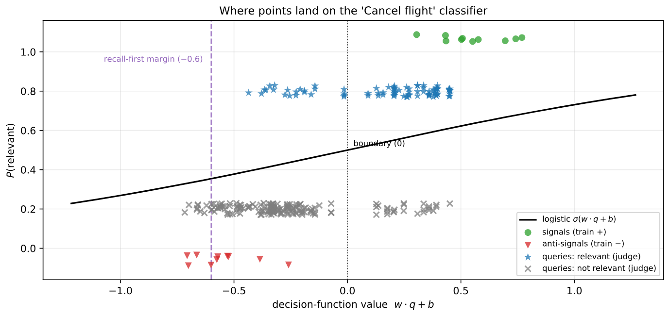
This figure shows the core difficulty of the whole paper. Generated exemplars separate perfectly on the classifier, yet real conversations all land between them, with relevant and irrelevant ones overlapping heavily. To miss as few relevant conversations as possible, the threshold has to go negative (−0.45 for Gemini, −0.4 for OpenAI, so a relevance probability of about 0.4 still passes), and many irrelevant conversations get through as a result. That is the root of the roughly one-third precision: there is a clear distribution gap between generated exemplars and real conversations.
3. Experiments
3.1 Setup
The data are 50 airline customer-service conversations produced by a Parlant agent against the τ²-bench user simulator. Every prefix ending at a user message is one query state, 254 in total. There are 36 rules: the 6 sections of τ²-bench's airline policy plus 30 written by the authors (identity verification, baggage claims, unaccompanied minors, fare rules, fraud handling and so on), deliberately including several near-synonym clusters. Ground truth comes from gemini-3.1-flash-lite, which uses Parlant's production relevance prompt to score every (conversation prefix, rule) pair from 1 to 5; a score of 4 or above counts as relevant, giving 9,144 labels. Metrics are macro-averaged over the 31 rules that occur at least once. There are four baselines with two kinds of score: the cosine between the query and the rule text, or the largest cosine between the query and the rule's 10 signals. Each is used either to take the top K rules or with a cosine threshold. The baselines use the same two query vectors and the same max as S&Q.
3.2 Recall and precision
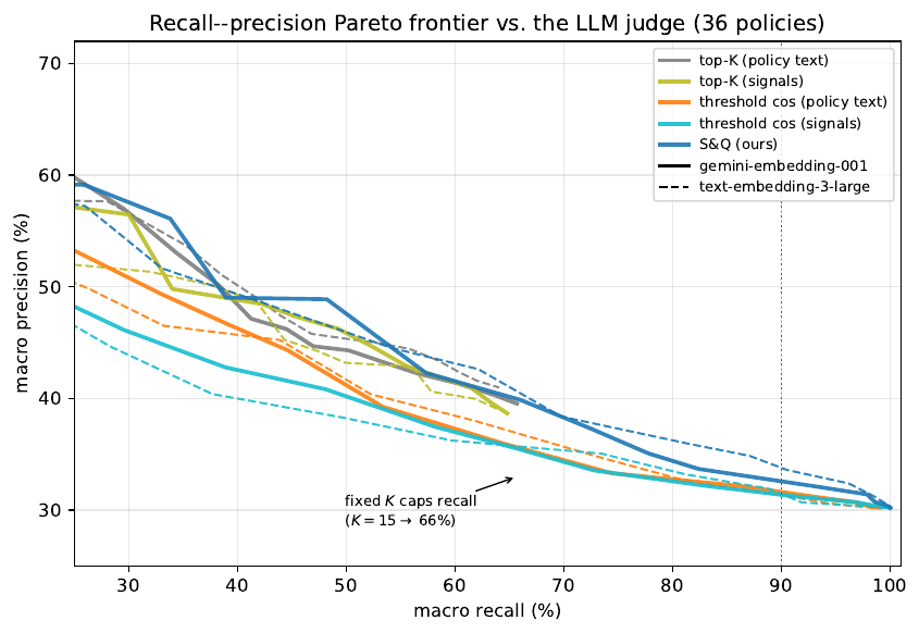
S&Q has the highest precision at every recall level and leads by about 4 points in the 60–70% recall range. At the high-recall end that actually matters, the gap shrinks to 2.9 points on OpenAI and 0.9 on Gemini. Top-K methods reach only about 66% recall even at K=15 (15 of 36 rules), because the number of rules relevant at the same time varies a lot from turn to turn, so a fixed-count cutoff is a poor fit for this task.
| Method | Gemini recall % | Gemini precision % | OpenAI recall % | OpenAI precision % |
|---|---|---|---|---|
| Top-K (rule text, K=15) | 66 | 40 | 64 | 41 |
| Top-K (signals, K=15) | 65 | 39 | 64 | 39 |
| Cosine threshold (rule text) | 93 | 31 | 94 | 31 |
| Cosine threshold (signals) | 91 | 31 | 92 | 31 |
| S&Q | 93 | 32 | 91 | 34 |
At the 90%-recall operating point, S&Q is only 1 to 3 points better than the simplest cosine threshold. In other words, with the default setup, training classifiers buys very little. The headline contribution, "better than embedding retrieval", is not significant at the deployment operating point.
3.3 Ablations: almost nothing matters
| Variant | Area under curve (Gemini) | Area under curve (OpenAI) | Precision at 90% recall (G/O) |
|---|---|---|---|
| Default | .471 | .475 | 32 / 34 |
| Negatives = other rules' signals | .501 | .498 | 32 / 33 |
| No negatives (no classifier; score by similarity to the nearest signal) | .423 | .429 | 31 / 31 |
| Whole-conversation view only | .526 | .531 | 34 / 34 |
| Linear SVM | .463 | .473 | 32 / 33 |
| Signed k-NN (nearest exemplars vote, signals positive, anti-signals negative) | .399 | .396 | 30 / 30 |
| 5+5 exemplars per rule | .436 | .436 | 31 / 33 |
"Area under curve" is AUPRC (area under the recall–precision curve), which covers the whole curve. The last column shows that every variant lands between 30% and 34% precision at 90% recall. Swapping in an SVM, dropping centering or halving the exemplars all give about the same result. Logistic regression and a linear SVM learn directions with cosine similarity 0.98, essentially the same classifier. Raising each rule's anti-signals from 10 to 30 moves precision from 32.4% to 32.3%. The reason is that 94% of the new exemplars have cosine similarity of at least 0.6 to one already present: the generator keeps writing similar sentences.
Two results run against the default setup. Using other rules' signals as negatives gives a slightly higher AUPRC than the dedicated anti-signals; the authors keep the latter to avoid the mutual suppression from Section 2.2. The whole-conversation view alone also scores higher, because the benchmark's conversations are short and single-topic (median about 1,600 characters), so the per-message max never gets to help. The authors therefore ran a synthetic test that stitches two different-task conversations into one "A then B" dialogue. At a 30% false-positive rate, the per-message max recovers 12 to 19 more points of recall on topic B's rules than the whole-conversation view. So this design may matter in real long conversations, but on the paper's main benchmark it is a slight drag.
3.4 Exemplars from real conversations
If the classifier, the encoder and the exemplar count do not matter, what is left is where the exemplars come from. The authors split the conversation scenarios in half and mined exemplars from one half. An LLM judge scores the rule's relevance turn by turn; the user message at which that score first reaches its maximum for the conversation, the message that actually triggered the rule, became a signal. A user message judged clearly irrelevant and closest to the rule's signals became an anti-signal. Evaluation is on the other half. In the table, the left of each arrow uses exemplars the LLM generated from the policy text (the earlier method) and the right uses mined exemplars, with everything else unchanged. SetFit in the last row is a few-shot classification method: it first fine-tunes a sentence encoder contrastively on a few labeled examples, then trains a classification head on the tuned vectors; here it tests whether fine-tuning the encoder beats S&Q's frozen one.
| Method | Precision at 90% recall (%) | AUPRC |
|---|---|---|
| Cosine (signals, Gemini) | 32.0 → 35.3 | .459 → .501 |
| Cosine (signals, OpenAI) | 32.8 → 36.5 | .467 → .480 |
| S&Q (Gemini) | 33.9 → 43.5 | .475 → .602 |
| S&Q (OpenAI) | 35.3 → 41.6 | .496 → .608 |
| S&Q (local MiniLM) | 32.6 → 39.7 | .457 → .540 |
| SetFit fine-tuned (local MiniLM) | 31.6 → 37.3 | .450 → .559 |
This is where the gap opens. With the same mined exemplars, cosine methods gain only 3 to 4 points of precision, while S&Q gains 6 to 10. Cosine similarity can only use positives and has nowhere to put a negative, and S&Q's gain comes almost entirely from the mined hard negatives. Replacing only the positives moves precision by +0.5 points on Gemini and −1.5 on OpenAI. With the same small local model, all-MiniLM-L6-v2, a frozen encoder plus logistic regression also gains more than SetFit, which fine-tunes the encoder. SetFit also means deploying one model of about 90 MB per rule, against about 12 KB of logistic-regression weights. The evaluation set, however, is only 131 conversation states, and the authors admit these results show direction and rough magnitude only.
4. Limitations
The authors list several limitations. There is one domain (airline) and one conversation source (τ²-bench simulations). 5 of the 36 rules never occur and cannot be evaluated. θ was chosen on this benchmark rather than derived from the rules themselves. And each rule's relevance is decided independently, so a dependency like "rule B applies only after rule A fires" is not handled, which the authors think belongs in a higher orchestration layer.
There are a few more. First, ground truth is another LLM's judgment with no human check, and S&Q exists to replace that very judgment, so the paper really measures how well it reproduces the LLM judge. Second, even in the best setup precision is only about 40%, so more than half of the surviving rules are irrelevant. That is fine when three to five rules come through per turn, but with hundreds of rules the surviving set may still be large. Third, mining needs relevance labels on real conversations. With the half-and-half split, only 22 of the 29 occurring rules had enough mined material, so a cold start must rely on generated exemplars, the one-third-precision level. The two kinds of exemplars also cannot be mixed. The authors found that training on generated and mined exemplars together cancels the gain. The classifier then learns "synthetic text versus real conversation" instead of this rule versus its neighbours. Fourth, in a long conversation a rule stays retrieved once it fires, so the retrieved set only grows, and a deployment needs a separate expiry mechanism.
5. Practical implications
When building an agent with many rules, tool descriptions or skill descriptions, you can replace "ask the LLM each turn whether this rule applies" with one offline-trained linear classifier per rule, cutting run-time cost to one embedding call. The authors also point out that the same method applies directly to filtering a skill library: skill names and descriptions sit in the context permanently, and once a library reaches hundreds of skills that alone becomes a burden.
The most important takeaway is where to invest. Changing the encoder, changing the classifier or adding more exemplars does nothing. What works is negatives, ideally ones mined from real conversations that are easily confused with a neighbouring rule. So after launch, set up a loop early: log every turn, have an LLM label relevance offline, and periodically mine new negatives and retrain. Since fitting each rule's classifier takes milliseconds, this loop is cheap to run.
How did this read for you?
Hoot made a note. Thanks for the feedback.

One tap, no sign-in; tap again to undo. Only anonymous counts are kept, never who you are.
Discussion
Add experiment details, reproduction notes or a different take. Requires a GitHub sign-in.
Loading the discussion…