Contents · 10 sections
1What problem is it actually solving?2The pipeline: one change per stage3Vocabulary: make valuable long-tail queries shorter4Location and time: from city tokens to continuous coordinates5Training: align directly on online impressions and clicks6Decoding: add a bonus only to the lower beams7Is the whole thing really better?8Where I think it falls short9How a recommendation or search team could try it10VerdictSHARE

Teams working on local-services or location-aware recommendation should read this: it builds one generative model for homepage query suggestions, with an online A/B test. The homepage of a local-services app must generate a few queries out of millions of possibilities, with no two alike, matching where the user is right now. SPADE (the generative framework in this paper) changes one thing in each of four stages of the generation pipeline. At tokenization, BPE weights fragment-pair counts by query click and conversion value, prioritising merges within valuable queries so long-tail queries become shorter. At the input, the user's exact coordinate and the current hour are encoded as vectors and added in. In training, it aligns directly on production impression and click data with DPO. At decoding, beams are ranked by cumulative score and receive a larger bonus further down the ranking, giving different queries more chance to survive. Offline, HR@5 is 5.6% higher (relative) than the strongest generative baseline, and the average distance from the user to the recommended shops is 40.3% shorter; in a one-week online A/B test, module CTR rose 1.88%.
I think the most useful part of this paper is that it splits one generation pipeline into four stages, changes one thing in each, and each change can be lifted out on its own. The four are the tokenizer vocabulary, how location and time enter the input, preference training, and decoding. The decoding change is the cheapest: you can try it without retraining. Each change targets one specific problem rather than a vague "stronger model". The ablation table shows which metric each piece mainly moves: the location encoding mainly drives distance, the decoding change mainly drives diversity.
What problem is it actually solving?
Query recommendation (the paper calls it proactive query recommendation) sits on the homepage of a local-services app. Before the user types anything, the system shows a few search queries under the search box, and tapping one runs that search. It differs from ordinary recommendation: ordinary recommenders pick from a fixed item pool, while here the system generates free text out of millions of platform queries, and each generated query must return suitable results in the platform's search engine.
An example (illustrative): at noon on a weekday, a user opens the app in an office district; they recently searched for hot pot and coffee. There are only 5 slots.
| Approach (illustrative) | 5 queries | Problem |
|---|---|---|
| Plain beam search | hot pot nearby, nearby hot pot place, good hot pot around, hot pot restaurant, hot pot rec | all 5 say the same thing |
| City-only location | hot pot, KTV weekend deal, hot-spring resort | the resort is tens of kilometres out; results are too far |
| Ideal | hot pot nearby, weekday lunch set, cafe for working, massage nearby, Japanese dinner | one distinct need per slot, all nearby |
The table shows two problems directly (repetition, coarse location); add two more and you have the paper's four requirements. First, long-tail queries are hard to generate: a rare query like "cafe for working" is cut into many tokens, and its generation probability is multiplied down step by step. Second, location is too coarse: putting only city and district into the input as text tokens cannot tell a district centre from its edge. Third, preferences do not match: generic preference training differs from the real impression and click distribution online. Fourth, decoding repeats itself: beam search ranks by probability alone, so the 5 outputs are often rewordings of one intent.
The pipeline: one change per stage
SPADE is a Transformer generation model. Its input sequence is, in order, the user profile, coarse context tokens (city, district, weekday, time slot and so on) and the last 30 behaviours (queries searched, names of shops visited); its output is 5 queries. The four changes, in pipeline order:
| Stage | Change | Problem it fixes |
|---|---|---|
| Vocabulary (before training) | OA-BPE: weight each query by business value during BPE merging | long-tail queries split too finely |
| Input | STAR: encode the exact GPS coordinate and hour as a few vectors added to the input | location only at city level |
| Training | cross-vertical pre-training, then MARS-DPO alignment on online impression-click data | preferences off the online distribution |
| Decoding (inference) | SDBS: give lower-ranked beams a bonus that grows with rank | repeated outputs |
The division of labour in one sentence: the first three changes decide how much probability the model gives each query, and the last decides how to pick 5 non-repeating queries from those probabilities. The sections below take them in order.
Vocabulary: make valuable long-tail queries shorter
Why would tokenization affect recommendation? The probability of generating a query is the product of its token probabilities, and each factor is at most 1. The more pieces a query is cut into, the more factors are multiplied and the lower the whole probability usually is. When tokenization follows frequency alone, rare long-tail queries stay finely split and start at a disadvantage when generated.
OA-BPE changes only the merge score. Standard BPE compares a fragment pair's total occurrence count in the training corpus. OA-BPE also considers the business value of the queries containing those occurrences: take their occurrence-weighted mean value and multiply it by the total count. The paper writes this as a weighted sum; equivalently:
Here is the pair's total occurrence count in the tokenizer's training corpus, and is the mean business value across those occurrences. This corpus count is not simply the online impression volume. Business value combines query CTR, CVR and an exposure-normalisation term, so exposure affects the weight. When every occurrence has weight 1, the score reduces to standard BPE.
A worked example (illustrative): pair A occurs 1000 times in queries with mean value 0.2, scoring 200; pair B occurs only 300 times with mean value 0.8, scoring 240. Standard BPE merges A first; OA-BPE merges B first. The paper states the simple rule behind this: a pair that is several times more valuable can overcome being that many times rarer.
This step runs once before training and adds no training or inference cost. The effect shows in tokenization statistics:
| Query type | Metric | Standard BPE | OA-BPE |
|---|---|---|---|
| Head (≥1000 occurrences) | median token count | 4.1 | 4.0 |
| Long tail (<100 occurrences) | median token count | 7.2 | 5.9 |
| Long tail (<100 occurrences) | probability of appearing in top-10 outputs | 0.312 | 0.383 |
The median token count of long-tail queries falls by 18.3%, and 64.1% of long-tail queries lose at least one token. Head queries barely change. This means the weighting changes how the long tail is split without breaking common queries.
Location and time: from city tokens to continuous coordinates
Why is this step needed? Writing a city ID as a token caps precision at that ID, and two IDs carry no notion of near or far. Local services care most about exactly the difference within a few kilometres.
STAR (the module that feeds location and time into the model) encodes the user's exact current coordinate and the current hour as a few vectors and adds them to the reserved positions at the start of the context segment of the input (the paper calls the number of vectors K, unrelated to the number of outputs):
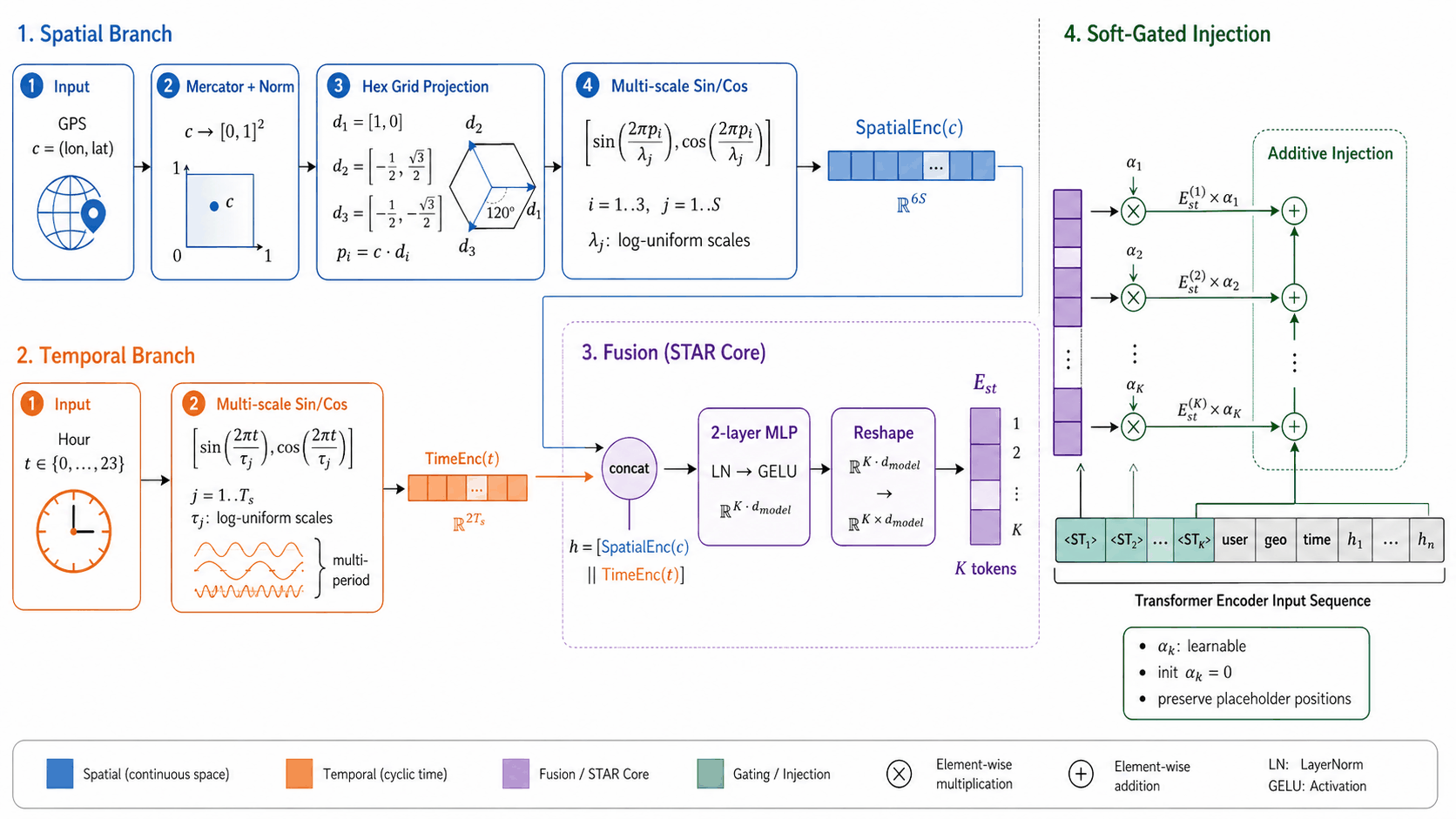
One way to picture the spatial encoding: draw over the map three sets of ripples, one along each of three directions 120° apart, with periods from about 1 km up to city scale. The user's readings on each set of ripples (the sine and cosine values) are concatenated into the code for that location. Short-period ripples separate neighbouring blocks; long-period ones separate city from suburb. The time encoding does the same for the hour of day. The two codes are concatenated, passed through a two-layer MLP, and split into these vectors.
Before each vector is added to the input, it is multiplied by a learnable gate initialised to 0. So at the start of training STAR has no effect and the model first learns the language part; as training goes on the gates grow and location and time signals come in gradually. The vectors are added to the reserved positions rather than replacing those positions' embeddings, so the original position encoding is kept.
Removing parts of STAR gives the following (GeoC@5 is the paper's geo-consistency metric: for each generated query, take the distance from the user to the nearest shop in its search results, then average; in km, lower is better):
| Variant | HR@5 | GeoC@5 (km) ↓ |
|---|---|---|
| Full SPADE | 13.2 | 1.66 |
| No spatial encoding | 12.7 | 2.55 |
| No temporal encoding | 13.0 | 1.79 |
| Single 1 km scale | 12.9 | 1.91 |
| No gate, direct addition | 12.8 | 1.82 |
Without the spatial encoding, GeoC@5 rises by 53.6% and HR@5 also drops by 3.8%. This shows location decides not only how near the recommendations are but also how accurate they are. Without the gate, both signals are still present, yet HR@5 falls to 12.8, which means pouring these vectors in early in training disturbs representations the model has already learned. As the finest scale goes from city level down to 1 km, GeoC@5 falls steadily from 2.68 to 1.66.
Training: align directly on online impressions and clicks
Training has two stages. The first is cross-vertical pre-training: on search logs across restaurants, entertainment, lifestyle services and other verticals, the model learns to predict the user's next search. Its cross-entropy first divides the model's score for each token by a temperature of 2, then computes probabilities and the loss, which makes the predicted distribution flatter.
The second stage is MARS-DPO (the paper's name), DPO on the impression-click data of the homepage query-recommendation module itself. It differs from standard DPO in three ways.
First, preference pairs come straight from the online candidate list. For each request, the online system has already recalled a batch of candidate queries. MARS-DPO picks positives and negatives from that batch, so no extra generation is needed and the training distribution matches online traffic.
Second, each candidate's reward is a weighted sum of three parts, with weights 0.8, 0.1 and 0.1:
| Reward | How it is computed | Weight |
|---|---|---|
| Rank position | where the online ranker placed it: rank r scores , so nearer the top scores higher | 0.8 |
| Searchability | give the query and its top results to Qwen3.5-122B-A10B, ask whether the query returns suitable results, read the probabilities of the answers "yes" and "no", take the share of "yes" | 0.1 |
| Distance | take the log of the distance from the user to the closest returned shop, min-max normalise it to 0–1 across candidates, subtract from 1; nearer scores higher | 0.1 |
All these rewards are computed offline before training. At serving time no LLM is called and no rewards are needed.
Third, negatives are chosen to be "hard". The highest-reward candidate is the positive; the rest are sorted by their reward gap to the positive, and the 5 with the smallest gaps become negatives. The smaller a negative's gap, the larger its weight in the loss. An example (illustrative): the positive has reward 0.9 and two negatives have 0.8 and 0.5, gaps 0.1 and 0.4. With the paper's concentration parameter of 2, the weights are in the ratio , about 65% to 35%, so the first negative counts more. The model thus mainly learns to separate the good from the nearly good, not pairs that are already easy to tell apart.
There are two smaller touches. Pure DPO can push both positive and negative probabilities down, so an SFT loss on the positive, weight 0.5, holds the positive's probability up. Each training sample is also weighted by feedback strength: impression without click 0.5, click 1.0, conversion 2.0. Hoot says

Before (illustrative)
- Positive probability
- 0.4
- Negative probability
- 0.2
- Positive / negative
- 2
One possible update (illustrative)
- Positive probability
- 0.3
- Negative probability
- 0.1
- Positive / negative
- 3
Illustrative: if the negative probability falls faster, the positive-to-negative ratio rises even while the positive probability falls. With the reference model fixed, this follows the direction of improved DPO preference. The positive SFT term separately encourages the positive probability to rise. These are not experimental results.
Source
Positive SFT term in §3.4.2; illustrative probabilities, ratios recomputed in checksReplacing MARS-DPO with standard DPO (random negatives, equal sample weights) lowers HR@5 from 13.2 to 12.8. Put the other way, MARS-DPO is 3.1% higher than standard DPO on HR@5 and 3.5% higher on MRR@5.
Decoding: add a bonus only to the lower beams
The first three changes shape probabilities; decoding picks 5 non-repeating queries from them. Decoding by probability alone, the 5 results are often rewrites like "hot pot nearby" and "nearby hot pot place".
SDBS (the decoding method that keeps outputs from repeating) is used only at inference. At each step the current B beams are ranked by cumulative score, with the top one as rank 0. Each beam expands 2B candidate tokens. A candidate's score is its parent beam's cumulative search score (log probability accumulated along the path, plus bonuses from earlier steps), plus the token's log probability, plus the bonus for the parent's rank. Candidates from all beams are sorted together and the top B become the next beams. The bonus curve is:
With , and , the curve has four properties. First, rank 0 gets exactly zero bonus. Second, lower ranks get more. Third, each further rank adds less than the one before. Fourth, the bonus has a ceiling of . sets the overall strength, 0.4 in production; sets how fast the bonus grows, and sets the ceiling's share of . Rank 0 getting no bonus does not by itself keep it on top: other beams may overtake it after their bonus. The paper's condition compares expanded candidate scores. The top beam gets no bonus, and every other candidate gets at most the ceiling. So if the top beam's best candidate leads every other beam's best candidate by more than that ceiling, it stays first, as in standard beam search.
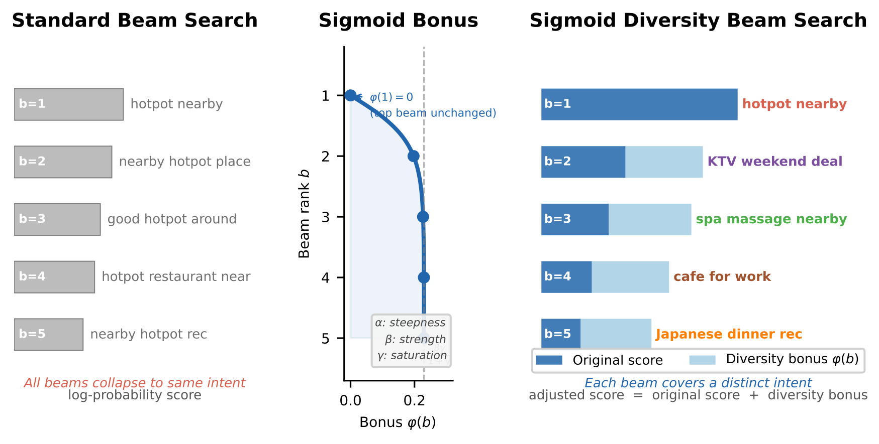
Why does a bonus bring diversity? Some of the pruned candidates are a different need, cut only because their original score fell slightly short. Topping up the lower-ranked beams gives their continuations a chance to survive. This is an intuitive explanation; the paper does not count how many rescued candidates are new needs. This differs from the existing Diverse Beam Search (DBS). SDBS never compares how similar two outputs are. It looks only at rank, so the extra cost of the bonus step grows only linearly with the number of beams; expanding and selecting candidates costs the same as in standard beam search. Also, DBS directly changes the top beam's score, while SDBS gives the top beam a bonus of 0 and leaves its score alone, although its continuation can still be overtaken by other beams.
The paper analyses a simplified model: if candidate scores fall with rank as a power law, then rescuing even the first pruned candidate needs a bonus larger than the gap between first and second place. The paper concludes that, in this simplified model, the conflict between diversity and relevance is set by the score distribution itself and cannot be tuned away. The paper also says this analysis only guides the curve's shape and parameters and does not guarantee results on real generated sequences.
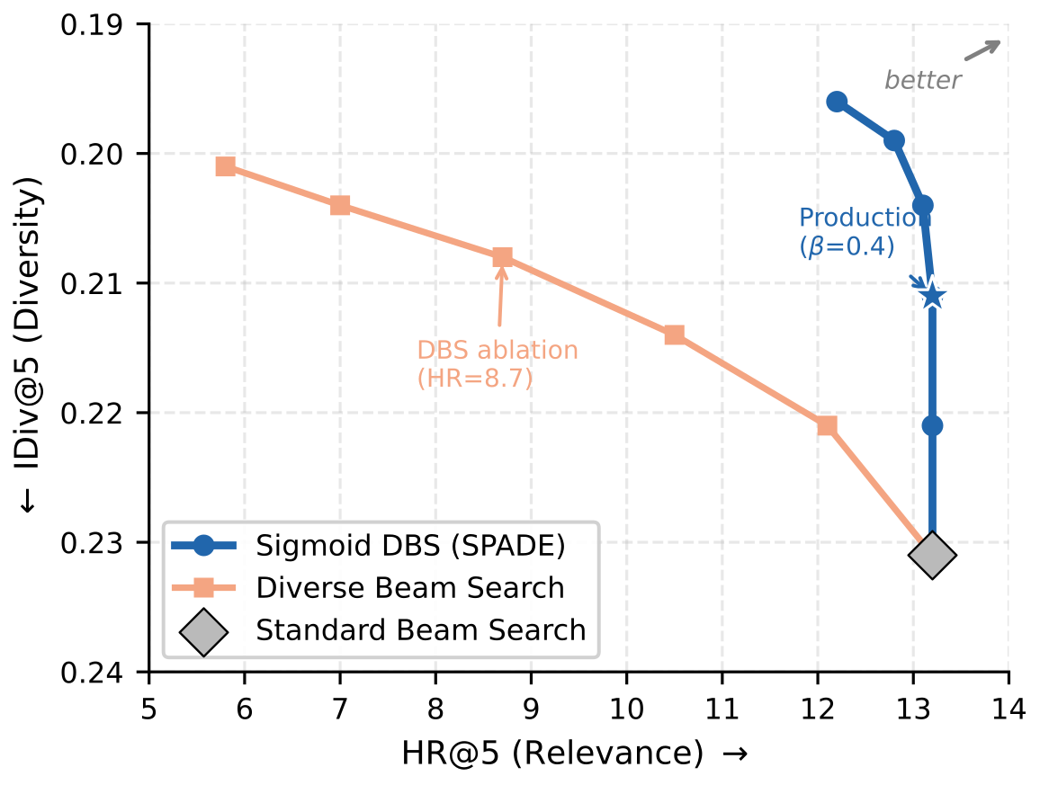
IDiv@5 in the figure averages pairwise cosine similarities between query embeddings to measure how alike the queries are; lower is more diverse. At the production setting, SDBS lowers IDiv@5 from standard beam search's 0.231 to 0.211, a drop of 8.7%, with HR@5 unchanged. DBS reaches a slightly better IDiv@5 of 0.208, but its HR@5 falls to 8.7, 34.1% lower, and GeoC@5 becomes 2.82 km. Touching only the lower beams buys diversity at almost no cost in relevance, which is why it can ship.
Is the whole thing really better?
The offline data come from a large local-services platform: 100K randomly sampled users, 30 days of logs for training, day 31 for validation and day 32 for testing, with 1.48M distinct queries and 2,608 cities. Baselines include non-generative production methods (such as SwingQ2Q, query-to-query recommendation on a search co-occurrence graph) and several generative methods. The strongest is AIGQ (an industrial generative query-recommendation method), which trains on whole lists and then optimises with reinforcement learning. Generative baselines that need fine-tuning are retrained on the same 30-day data under their own original training objectives; the zero-shot LLM baseline is not trained. All methods get the same input features, including exact coordinates. On the input side, AIGQ and others write location and time as text tokens, while SPADE uses continuous encodings. At evaluation, the target is the query the user actually searched on the test day. Exec@5 is a searchability score: a different LLM, Qwen3-32B, judges whether each query returns suitable results, scored 0 to 1. It is not the model used for the training reward, and its prompt was written separately.
| Method | HR@5 | MRR@5 | IDiv@5 ↓ | GeoC@5 (km) ↓ | Exec@5 |
|---|---|---|---|---|---|
| SwingQ2Q | 9.7 | .0738 | .279 | 2.31 | .897 |
| OneSug | 11.3 | .0891 | .234 | 3.05 | .903 |
| Local-SUG | 11.0 | .0867 | .241 | 2.28 | .915 |
| AIGQ | 12.5 | .1012 | .204 | 2.78 | .934 |
| SPADE | 13.2 | .1065 | .211 | 1.66 | .952 |
SPADE's HR@5 is 5.6% above AIGQ in relative terms (12.5 to 13.2), its GeoC@5 40.3% lower, and its Exec@5 1.9% higher. This shows the lead is largest on distance and much smaller on relevance. The biggest change is in GeoC@5: the recommended shops are on average more than 1 km closer to the user, which is exactly what STAR is for. The only metric it does not win is diversity: IDiv@5 is 0.211, slightly worse than AIGQ's 0.204. The paper's explanation: AIGQ sees the queries already generated when producing each new one, so it deduplicates naturally; SPADE scores each candidate separately during training without seeing the others in the same list, so diversity is left to decoding. Without SDBS, IDiv@5 is 0.231 and the gap would be wider.
By traffic slice, SPADE's lead grows in the harder cases: on long-tail queries HR@5 is 13.5% above AIGQ in relative terms (7.4 to 8.4), on new users with fewer than 5 behaviours 9.8% above, and in sparse regions with under 10K monthly active users GeoC@5 is 48.3% lower. At weekday meal hours (11–13 and 17–20) the GeoC@5 gap narrows to 28.1%, because lunch near the office is routine and coarse location is already enough.
A one-week online A/B test checks whether the offline gains carry over, with 20% of traffic per arm: module CTR rose 1.88%, search volume 0.177% and search DAU 0.105%, all significant. On a single inference GPU the model takes about 20 GB of memory, serves 289 QPS, with P50 latency 36.1 ms and P95 65.4 ms, within the platform's 100 ms limit and with no extra GPUs. The four changes together did not raise serving cost.
Where I think it falls short
First, each component's own contribution is small, and the ablation has no significance test. Without OA-BPE HR@5 is 12.5, without STAR 12.6, with standard DPO 12.8, only 0.4 to 0.7 points below the full 13.2. In other words, each component adds less than 1 point of HR@5. Significance is tested only in the main table (SPADE against AIGQ), so whether a single component's gain reproduces on another platform has to be measured yourself.
Second, diversity still loses to AIGQ: IDiv@5 is 0.211 against 0.204, because MARS-DPO scores candidates one by one and never sees the whole list. If a product cares a lot about differences among the 5 queries, decoding alone will not close the gap.
Third, several parameters needed for reproduction are missing. Reproducing the method also needs the mix of CTR, CVR and the exposure term inside the business-value weight , and SDBS's and , which are left out of the paper's settings. The OA-BPE weights also need periodic recomputation as the query distribution shifts, which the authors note themselves.
How a recommendation or search team could try it
- Start with SDBS. It changes only inference-time decoding, with no retraining. Add the bonus curve to your existing beam search, sweep upward from small values while watching HR@5 and within-list similarity, and pick the point just before HR@5 starts to fall.
- Then try OA-BPE. Weight queries by CTR and CVR, retrain the tokenizer, and first check only tokenization statistics: are long-tail queries shorter, and are head queries essentially unchanged? A new vocabulary means retraining the model, so confirm the statistical gain first.
- Add STAR for location-sensitive scenarios. Feed the exact coordinate into the input with multi-scale sinusoidal encoding and zero-initialised gates, and watch distance-type metrics and the sparse-region slice.
- Do MARS-DPO once you have impression-click logs. Start with rank position as the only reward and pick hard negatives from the same request's candidates; once that beats random negatives, add the searchability and distance rewards.
Verdict
The key lesson: in generative recommendation, the vocabulary and the decoder are not neutral infrastructure; they themselves decide which queries are easy to recommend.
| Dimension | Assessment |
|---|---|
| Problem importance | High. Homepage queries are the entry point of local-services search traffic, and long tail, location and repetition are real problems |
| Method novelty | Medium. None of the four changes is complex; the value is aiming each at a concrete failure and combining them in one pipeline |
| Evidence | Medium-high. Offline main table, ablations, slices and a one-week online A/B; ablation gaps are small and untested for significance |
| Engineering cost | Medium. SDBS is nearly free; OA-BPE and STAR need retraining; MARS-DPO needs offline LLM searchability scoring |
| Worth trying | Yes. Start with SDBS; the lists become more diverse at almost no cost |
| Fits | Query recommendation, query autocomplete, any setting that generates a few short texts at once and cares about location |
How did this read for you?
Hoot made a note. Thanks for the feedback.

One tap, no sign-in; tap again to undo. Only anonymous counts are kept, never who you are.
Discussion
Add experiment details, reproduction notes or a different take. Requires a GitHub sign-in.
Loading the discussion…