Contents · 9 sections
1What problem is it solving?2The big picture3Where the two SIDs come from4The decoder: generate the two SIDs interleaved, then extract representations with task queries5Offline experiments: above the online baseline, but by small and uneven margins6Online results and cost7Limitations as I see them8How a recommendation team could try it9Bottom line and assessmentSHARE

This is worth reading for recommendation teams working on live streaming, e-commerce, or any setting where item content changes in real time. It does not take the route of having a generative model emit recommendations directly. Instead it puts a generative encoder–decoder on the user side of a pre-ranking model, uses it only to generate Semantic IDs and extract user representations along the way, and leaves final scoring to a discriminative network with cross features. The core idea in one sentence: each live room gets two SIDs. One comes from the streamer's content over the past few days and barely changes; the other is quantized from the room's real-time features and changes with the content. The decoder generates the two SIDs in an interleaved order, then a few learnable queries per task extract representations, which are combined with user–streamer cross features such as likes and orders for multi-task prediction. In the online A/B test, watch time rose 3.38% and GMV (gross merchandise value) rose 0.72%; model compute went from 0.9T to 15T FLOPs, while latency rose only 1.33%. I think the split into a static SID plus a dynamic SID is worth borrowing, but the offline gains are small and uneven, and the evidence for the dynamic SID is a single live-room case.
What problem is it solving?
Start with an illustrative scenario. A clothing streamer goes live at 8 pm and spends the first half hour chatting to warm up, with few viewers. At 9 pm new jackets go on sale and the audience grows several times over. For a recommender, the same live room is two different things at these two moments.
Recommendation has recently adopted Semantic IDs (SIDs) to represent items: encode an item's multimodal content into a vector, then quantize it level by level into a few discrete codes, so similar items share prefixes. A short video's SID is static, because once posted its content does not change. Live streams are different, and the authors point out two issues:
| Difficulty | What it looks like |
|---|---|
| Content changes in real time | What the room talks about, sells, and how popular it is change all the time; a static SID can only describe the streamer's usual style |
| User–streamer interaction matters | Whether a user has liked or bought from this streamer is a strong signal for whether they will enter and buy; purely generative methods usually have no place for such cross features |
The other background is compute. The authors say their online pre-ranking model (DLRM, a conventional attention-plus-MLP design) is already strong, further architecture changes yield little, and compute utilization is low. Generative architectures improve when parameters grow, so the question is how to use one without losing cross features.
Pre-ranking here is the layer between retrieval and ranking: a two-tower model first encodes the user and the candidate separately, then a lightweight interaction network scores them. The user tower runs once per request, while candidate-side compute runs once per candidate, so heavy compute should sit on the user side.
The big picture
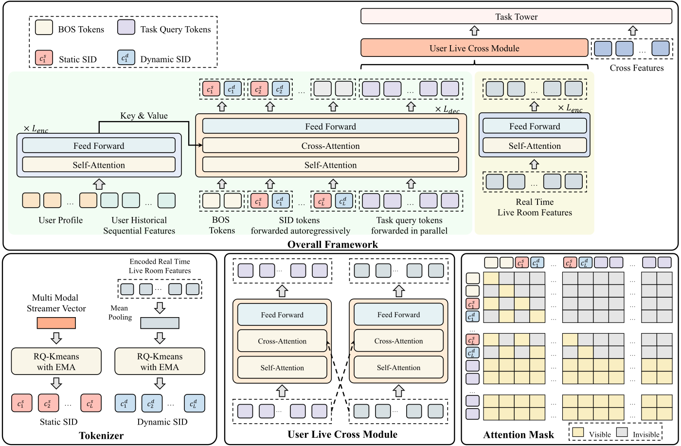
The pipeline splits into four steps:
| Step | Input | Output |
|---|---|---|
| 1. Build two SIDs | The streamer's historical segments over the last M days; the room's current real-time features | Static SID and dynamic SID, 3 levels each, 2,048 codes per level |
| 2. User-side encode–decode | User profile, behavior history | Generates the two SIDs interleaved, while task queries extract user representations |
| 3. User–live cross | User representation, live room real-time representation | Representations after mutual cross-attention |
| 4. Multi-task prediction | The previous step's representations + user–streamer cross features | Scores for watching over 30 s, over 200 s, ordering, and so on |
Where the two SIDs come from
The static SID describes what the streamer is usually like. The authors take the streamer's live segments over the last M days, sample several per day, and encode each with a fine-tuned multimodal model (these vectors are frozen during training). A Transformer encoder then aggregates them, and the mean gives the streamer vector. A pure content vector lacks collaborative signal, so Swing (an item-similarity algorithm common at Alibaba that checks whether two items are clicked by the same set of users) mines similar-streamer pairs for contrastive learning that pulls similar streamers' vectors together. Finally RQ-KMeans (residual quantization by repeated k-means: cluster at level one, cluster the level-one residuals at level two, and so on) quantizes it into 3 codes.
The dynamic SID describes what the room is like right now. Its input is real-time features, such as the current viewer count and the current segment's content. These features pass through an MLP projection and a Transformer encoder, are averaged into a real-time vector, and are quantized into 3 codes the same way. This encoder is initialized from an already trained live-streaming recommendation model so it converges faster.
The real-time vectors keep moving, and a fixed codebook cannot keep up, so the codebook is updated by EMA (exponential moving average). Each code keeps "the number of vectors assigned to it" and "the sum of those vectors". For each batch, both are updated as 0.99 of the old value plus 0.01 of the new one, and the code vector is their ratio. Here is a one-dimensional hand example. A code currently has count 100 and sum 100, so its value is 1.0. In a batch, 10 vectors are assigned to it, with mean 2.0 and sum 20. After the update the count is 0.99×100+0.01×10=99.1, the sum is 0.99×100+0.01×20=99.2, and the code value becomes about 1.001. This shows the codebook moves only slowly and no single batch can drag it, which buys stability.
Does the dynamic SID really follow the room? The paper gives one streamer at 3 moments in a day. The static SID stays (1512, 646, 631), while the first two levels of the dynamic SID go (111, 1559), (111, 1551), (111, 1194), and the 5-minute view count rises from under 100 to over 700. This shows that as popularity changes, the second level of the dynamic SID changes with it while the first level stays put, and the static SID does not react to these changes at all.
The decoder: generate the two SIDs interleaved, then extract representations with task queries
The user side is a standard encoder–decoder. The encoder reads the user profile and behavior history. The decoder input is, in order: two start tokens for static and dynamic; the two SIDs interleaved, that is, level-1 static code, level-1 dynamic code, level-2 static code, level-2 dynamic code, and so on; and finally 2 learnable query tokens per task.
Why interleave? Generating the full static SID before the dynamic one would take 6 autoregressive steps. Interleaved, each step produces the same level's static and dynamic codes together, so 3 steps suffice and generation time halves. To keep the two SIDs from interfering, the attention mask lets static codes see only earlier static codes and dynamic codes see only earlier dynamic codes. Task queries see all SID tokens and each other, and are computed together in one forward pass.
Training samples are individual user–live room interaction records. For the SID supervision, the paper uses next-token prediction cross-entropy over each level of the static and dynamic SIDs. As I read it, the target is the two SIDs of the live room in that record, which teaches the model from the user's history "what kind of live room this person will enter next". Training uses teacher forcing (each step is fed the true previous code rather than the model's own output). At inference there is no true SID, so beam search generates it. SSRLive keeps one beam set for static and one for dynamic, both of size 10. The b-th static candidate pairs with the b-th dynamic candidate; each sequence probability is normalized within its set, the pair's weight is the mean of the two, and the user representations of the 10 pairs are summed with these weights. A hand example with only 2 pairs: normalized static probabilities are 0.7 and 0.3, dynamic are 0.6 and 0.4, so the pair weights are (0.7+0.6)÷2=0.65 and (0.3+0.4)÷2=0.35. The benefit is that it does not bet on a single SID result; when generation is uncertain, the representation naturally blends several possibilities.
Task queries are the part that actually connects generation and discrimination. The decoder's last few outputs are the representations that each task's 2 queries extract from the SIDs and user features. The live room real-time branch is also projected into the same "number of tasks × 2" vectors. Each side first applies self-attention, then they cross-attend to each other, and finally the result is sliced by task, concatenated with user–streamer cross features, and fed to each task's MLP. Online, the task scores are multiplied with weights to give the final pre-ranking score.
Offline experiments: above the online baseline, but by small and uneven margins
The offline data is one week of Taobao Live, about 1 billion user–streamer interactions. There are three tasks: watching over 30 seconds (Watch30), over 200 seconds (Watch200), and placing an order (Order). Metrics are AUC and GAUC (AUC computed per user and then weighted-averaged, closer to "does it rank well for the same person"). Among baselines, DLRM is Taobao Live's online pre-ranking model; SASRec, ReaRec, and HSTU were originally retrieval sequence models, and the authors use their backbones to encode users and rooms, then attach the same cross features and MLPs to turn them into pre-ranking models.
| Model | Watch30 AUC | Watch30 GAUC | Watch200 AUC | Watch200 GAUC | Order AUC | Order GAUC |
|---|---|---|---|---|---|---|
| DLRM (online baseline) | 0.7610 | 0.6892 | 0.8229 | 0.7288 | 0.8312 | 0.6727 |
| SASRec | 0.7581 | 0.6781 | 0.8154 | 0.7105 | 0.8205 | 0.6689 |
| HSTU | 0.7613 | 0.6823 | 0.8192 | 0.7156 | 0.8249 | 0.6710 |
| SSRLive | 0.7692 | 0.6956 | 0.8255 | 0.7281 | 0.8358 | 0.6946 |
This table shows two things. First, the online baseline is strong: adapted models such as HSTU are worse than DLRM almost across the board, so moving a general sequence model over does not by itself add points. Second, SSRLive's gains concentrate on Watch30 and on Order GAUC, which rises 0.022; but Watch200 AUC rises only 0.0026, and its GAUC is even 0.0007 below DLRM.
| Ablation (component removed) | Watch30 AUC | Watch200 AUC | Order AUC | Order GAUC |
|---|---|---|---|---|
| Full SSRLive | 0.7692 | 0.8255 | 0.8358 | 0.6946 |
| No SIDs at all | 0.7602 | 0.8179 | 0.8245 | 0.6773 |
| No dynamic SID only | 0.7637 | 0.8214 | 0.8280 | 0.6798 |
| No task queries | 0.7676 | 0.8246 | 0.8344 | 0.6960 |
| No cross features | 0.7593 | 0.8149 | 0.8269 | 0.6826 |
This shows that SIDs and cross features are the two main pillars: removing either drops Watch30 AUC below DLRM's level. Removing only the dynamic SID loses about half to 70% of what removing all SIDs loses, which means the dynamic SID contributes a good share of the gain. Task queries matter much less, and Order GAUC is slightly higher without them. In the appendix, raising queries per task from 2 to 5 adds another 0.002 to 0.003 AUC on all three tasks, so this part still has headroom.
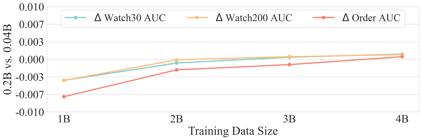
The figure above is the authors' answer to "does adding parameters help". It shows the larger model does need more data to catch up, but at 4 billion samples its lead is only about 0.001, and the deployed model is the small 0.04B version. So this paper's gains come mainly from the SID and cross-feature design, and the scaling payoff has not shown up yet.
Online results and cost
The online A/B test compares against DLRM, and every metric improves significantly:
| Metric | Gain |
|---|---|
| Watch time | +3.38% |
| Watch count | +1.89% |
| GMV | +0.72% |
| Order count | +2.36% |
| Follower count | +3.12% |
| Interacting users | +2.92% |
This shows the gain is not limited to offline AUC: from watching and buying to following and interacting, online metrics rise together, with watch time and follower count rising the most.
On cost, SSRLive has 0.04B dense parameters versus DLRM's 3M. The paper's efficiency table lists both models' dense compute on the same basis: 15T FLOPs for SSRLive and 0.9T for DLRM. The table gives only this one total, so only the ratio is used here: for the same online service, compute grows about 16 times. Latency rises only 4.41%, because the user-side generative module runs once per request, and the live room encoder does not depend on the user, so it runs asynchronously in an external service, refreshes only when the room's state changes, and is reused by tens of thousands of requests. With Partial Run (starting the user-side computation before candidate room data is ready), the latency increase falls to 1.33%. Putting heavy compute on the user side, which runs once per request, is the key to getting this architecture into pre-ranking.
Limitations as I see them
First, the offline gains are small and uneven. Among the three tasks, Watch200 GAUC is 0.0007 below the online baseline, and its AUC rises only 0.0026. The offline data covers only one week, the baselines are all adapted, and there is no public dataset, so it is hard for others to reproduce.
Second, the direct evidence for the dynamic SID is thin. Apart from the ablation numbers, the only demonstration that the dynamic SID follows the room is one streamer at 3 moments in a day. How often the dynamic SID refreshes, and whether an EMA codebook moving at 0.99 can keep up with minute-level changes in a live room, are things a team must measure at deployment.
Third, the scaling claim needs a discount. The larger model leads by only about 0.001 AUC at 4 billion samples, while the main offline experiment uses about 1 billion, and the deployed model is the small version. The online gains bought with 16 times the compute should be credited mainly to the SID and cross-feature design.
How a recommendation team could try it
- First check whether your items really "change in real time": for live rooms or other dynamic items, measure how much the same item's features (popularity, content) differ across times of day. If they barely change, do the static SID only.
- Add the static SID as an extra feature to your existing pre-ranking model and check offline AUC and GAUC.
- Then add the dynamic SID: use your existing model's item-tower output as the real-time vector, quantize it with RQ-KMeans, and update the codebook by EMA; also log how many times per day the same item's dynamic SID changes.
- Only then consider replacing the user side with an encoder–decoder plus task queries, together with the two engineering optimizations of running the user side once and caching the item side asynchronously; otherwise latency will eat the gains.
Bottom line and assessment
The most useful takeaway is that items whose content changes can be represented by a stable static SID plus a dynamic SID that follows real-time features, with the generative architecture only producing these two SIDs and user representations, while scoring stays with a discriminative network that has cross features.
| Dimension | Assessment |
|---|---|
| Importance of the problem | High. Live streaming, e-commerce sales events, and other real-time settings are common, and static IDs cannot keep up |
| Novelty of the method | Medium. The dynamic SID and interleaved generation are new; the rest combines existing parts |
| Experimental evidence | Medium-low. The online A/B is solid; offline gains are small with one metric below baseline, and the dynamic SID has a single case |
| Engineering cost | High. It needs two SIDs, an asynchronous live room encoding service, and early-start engineering changes |
| Worth trying? | Yes, starting by adding static and dynamic SIDs as features to an existing model |
| Where it fits | Pre-ranking or ranking for live streaming, real-time content feeds, and other items whose state clearly changes over time |
How did this read for you?
Hoot made a note. Thanks for the feedback.

One tap, no sign-in; tap again to undo. Only anonymous counts are kept, never who you are.
Discussion
Add experiment details, reproduction notes or a different take. Requires a GitHub sign-in.
Loading the discussion…