SHARE

Teaching a humanoid robot whole-body control by tracking large amounts of human motion data is currently very compute-hungry: the strongest motion tracker, SONIC (a previously released tracker trained with PPO on a cluster), trains for about 7 days on 128 GPUs. SuperMimic starts from a simple observation: the motions differ wildly, but the robot's body obeys one set of physics. It first learns a differentiable world model from simulator logs, then lets the policy imagine short rollouts inside that model and take gradients directly with respect to its actions. After 3 hours on a single GPU its return already exceeds SONIC's, using more than 1000× fewer GPU-hours. The bottleneck shifts from compute to the motion data itself, and adding more motions becomes cheap.
Recommendation and search engineers should read it too, because it answers a general question: when the environment cannot be differentiated and sampling is expensive, can you first learn a differentiable stand-in for the environment and backpropagate policy gradients straight through it? On a benchmark of 129,514 motions, SuperMimic after 3 hours on one GPU fails on only 25, against 179 for SONIC; after 9.8 hours on two GPUs it fails on none.
What problem is it actually solving?
Motion tracking works like this: the robot gets a piece of human motion capture (walking, a side roll, a flip). At every step it sees its own joint state and the next few reference frames, outputs joint targets, and tries to reproduce the motion without falling. The more diverse the data, the more general the controller.
The trouble is the training method. The mainstream approach uses model-free RL such as PPO, updating the policy through large amounts of trial and error in the simulator. PPO has no idea what the physics looks like, so for every motion it has to rediscover "what happens if I push this way" through lots of noisy trial and error. The illustrative table below shows where the waste is:
| Motion clip (illustrative) | What each clip must learn | What all clips share |
|---|---|---|
| Slow walk | Which leg to step with, and when | The same body's mass, joints, and foot–ground contact |
| Side roll | How the torso rolls along the floor | Same as above |
| In-place flip | Take-off force and landing | Same as above |
The right-hand column is identical for every motion, but PPO has nowhere to store it, so it re-estimates it inside each motion's trial and error. As the motion library grows from a few hours to hundreds of hours, compute has to grow with it. SuperMimic learns that shared column once as a separate model and lets every motion share it.
The whole pipeline: a three-step loop
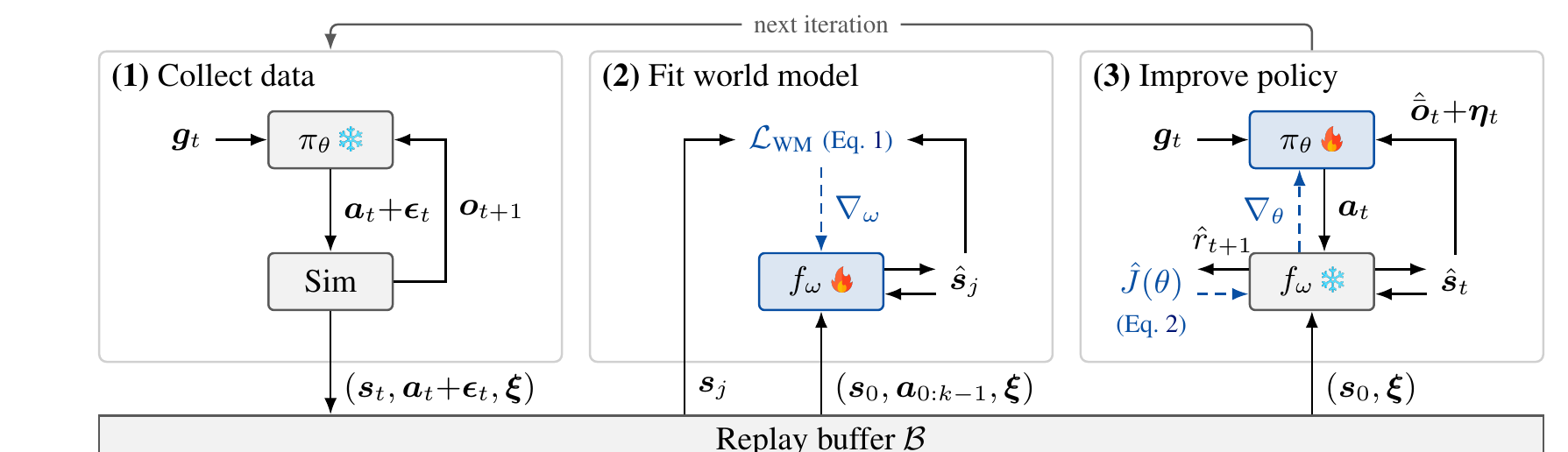
Training is a loop that repeats over and over, with three steps per iteration:
| Step | Input | What it does | Output |
|---|---|---|---|
| Collect data | Current policy, reference motion | Runs noisy actions in the GPU simulator MuJoCo Warp | States, actions and simulation parameters, written to the replay buffer |
| Fit world model | 8-step clips from the buffer | Starts at the clip's first state, predicts 8 steps in a row using the logged actions, compares with the log | Updated world model |
| Improve policy | Start states sampled from the buffer | World model frozen; the policy imagines 32 steps in it and differentiates the return with respect to the policy parameters | Updated policy and value network |
All three steps run every iteration, so the world model and the policy improve together instead of training the model first and the policy second. Data collected by older policies stays useful for fitting the world model, because the physics does not depend on which policy collected the data. Below we take the steps apart.
What does the world model learn, and how?
Why is it needed? The simulator can compute physics, but it gives no gradients, and contacts and collisions are not smooth anyway. SuperMimic learns a neural network as a stand-in for the simulator. Its core is the dynamics part: given the current state, the action and this episode's simulation parameters, it predicts the next state. Three output heads sit beside it. The reward head looks at the state, the action and the current goal (the corresponding frames of the reference motion), and scores how closely this step matches. The fall head looks at the state and the goal and gives a fall probability. The observation head looks at the state and the simulation parameters and gives the sensor readings the robot can see. The stand-in is an MLP with three layers of width 2048, so it is differentiable by construction. The simulator itself needs no changes, so the method works with any off-the-shelf rigid-body simulator.
The simulation parameters are the friction, sensor calibration offsets and torso center of mass randomly set for each episode. Randomness in the simulator comes only from these parameters and from sensor noise, so the authors feed the parameters directly to the world model. That keeps the model deterministic: it predicts noise-free readings, and the noise is added outside the model.
How is it trained? Take an 8-step logged clip from the buffer. Give the model only the true state at step 1; for the remaining 7 steps it rolls forward from its own previous prediction, while the actions follow the log. At each step the predicted state, reward and readings are compared with the true values by squared error, and the fall probability is matched with BCE. An illustrative case: if the predicted torso height is 1 cm off at step 1, step 2 continues from that biased state, and if the error snowballs, the loss grows. Making the model keep predicting from its own mistakes teaches it to pull the error back, which is why the authors observe that although it is trained on only 8 steps, imagining 32 steps or longer does not diverge.
How does the policy get its gradient from the world model?
This is the core of the paper. During a policy update the world model's parameters are frozen. A real state is sampled from the buffer as the start, together with that episode's recorded simulation parameters, which are used for the whole imagined rollout. The policy sees the model's readings (plus the same sensor noise as on the real robot) and outputs an action; the world model returns the next state and reward; this repeats for 32 steps, with each step's goal still being the corresponding frames of the reference motion. At a control rate of 50 steps per second, that is under one second. One step is left unexplained in the source: when imagination starts from a single buffer state, how the policy's last 10 frames of observation history and the matching reference-motion segment are prepared, and how they advance step by step.
The sum of the 32 rewards is the policy's objective. Because every step is a differentiable network, BPTT can backpropagate the return along the chain "reward ← state ← action ← policy parameters" all the way to the policy parameters.
An illustrative example makes the difference from PPO clear. Suppose one joint's reward is and the current action is . BPTT directly computes the derivative and knows in one step "turn it down". PPO never sees the formula; it has to try a few times, say 0.45 and 0.6, notice that the first got the higher return, and adjust from that, and with few tries the estimate is unstable. BPTT uses the direction of change for each action given by the world model, PPO uses a statistical estimate from trial outcomes, so over short horizons the former's gradient is far less noisy. Note that this direction is computed inside the learned stand-in: it approximates the gradient of the simulator's true return, and its accuracy depends on how well the world model has been learned. That is also why the world model is refit on fresh data in the same loop as the policy. Hoot says

PPO: compare tries
- try a=0.45
- reward −0.0225
- try a=0.6
- reward −0.09
- conclusion
- smaller is better; step size estimated from more tries
BPTT: differentiate directly
- tries needed
- none, one backward pass
- derivative
- −2(0.5−0.3) = −0.4
- conclusion
- turn it down; direction and size in one go
Illustrative: reward −(a−0.3)², current action a=0.5. Left compares the returns of two tries; right differentiates straight through the world model. BPTT's derivative is taken inside the learned stand-in, so its accuracy depends on the world model. Source: illustrative example for the paper's §3.3 contrast between BPTT and PPO
Falling must be differentiable too. In the simulator a fall is 0 or 1, and no gradient passes through. The world model instead predicts a fall probability, and a "survival weight" discounts later rewards: it starts at 1 and at each step is multiplied by (1 − that step's fall probability). Illustratively, with fall probability 0.1 at step 1 and 0.5 at step 2, the weight after two steps is 1 × 0.9 × 0.5 = 0.45, so later rewards count only 45%. To keep those later rewards, the gradient pushes the policy toward lower fall probability.
Why is a value network still needed?
Looking only 32 steps ahead has a problem: the payoff of getting up after a fall or recovering from a push often arrives after more than a second, beyond 32 steps. SuperMimic adds a value network (critic). It takes the predicted state at step 32, the goal and the simulation parameters, estimates "how much reward is still to come from here", and adds that after the 32 step rewards. The critic trains only on imagined trajectories. The value beyond step 32 is simply the critic's own estimate for the step-32 state; from there the targets are computed backward one step at a time, each equal to that step's reward plus the discounted value after it. The targets are fixed once computed, and the critic fits them. So although it only ever sees 32-step trajectories, its estimates pass payoffs from beyond the horizon back in, layer by layer.
The experiments show this step's effect clearly. First, how return is measured throughout: each step's reward measures how closely the robot's motion at that step matches the reference motion; the rewards of every step in an episode are summed and divided by the highest score attainable, so a perfect score is 1, and an episode that ends early in a fall naturally scores low. Without the critic, training fails at 16 imagined steps or fewer; with it, 16 steps match the critic-free 32 steps, and 32 steps reach the target return of 0.82 fastest. Longer is not better either: going from 64 to 128 steps nearly triples the time to the target and lowers the final return. The reason is that a longer backprop chain makes gradients less stable and memory tighter; 128 steps is the most one H100 can fit.
The critic also changes behavior. In simulation the robot holds a T-pose and is then pushed, with the push velocity raised from 0.5 m/s all the way to 4 m/s. The critic policy settles within 2.4 seconds every time; the critic-free one keeps stumbling even under a light push and falls under a hard one. Their returns on ordinary tracking are about the same, which shows the difference only appears when the policy needs to look further ahead.
One more small design: where in the motion library each simulator episode starts is chosen by return. The motion timeline is cut into 1-second bins, and the policy starts more often from bins where it earns low return, while half of the time it samples uniformly so it does not practise only hard motions.
Experiments: where do the compute savings come from?
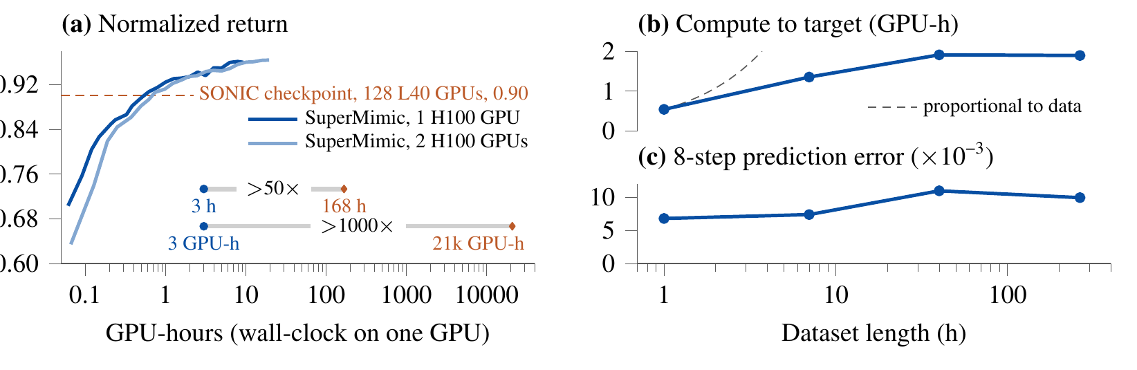
The main result compares against SONIC's released checkpoint, with both sides using the same motion-tracking reward:
| Metric | SONIC | SuperMimic 1×H100, 3 h | SuperMimic 2×H100, 9.8 h |
|---|---|---|---|
| Training compute | 128×L40, about 168 h, about 21,000 GPU-hours | 1 GPU × 3 h | 2 GPUs × 9.8 h |
| Failed motions (of 129,514) | 179 | 25 | 0 |
| Failed side rolls (of 22) | 22 | 2 | 0 |
| Failed flips (of 44) | 44 | 1 | 0 |
SONIC fails whole groups: all 44 flips and all 22 side rolls. SuperMimic's 25 failures after 3 hours on one GPU sit in a few groups of hard motions, and in no group does it fail more than SONIC. This shows the saved compute did not come at the cost of hard motions. The authors also spell out the differences in setup: SuperMimic uses only SONIC's public data subset, 264.56 hours, about 2.3× less than SONIC's 611 hours, and an H100's peak tensor-core throughput is 5.5× an L40's. Together these still cannot explain a 1000× gap.
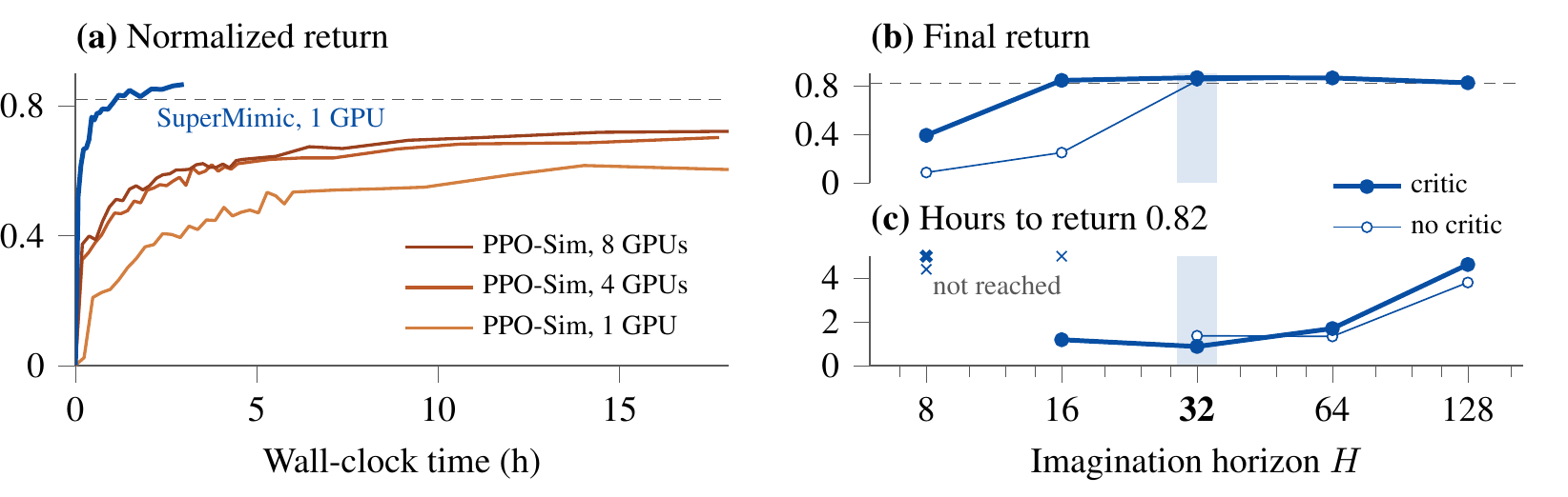
The SONIC comparison has too many variables, so the authors also ran a controlled experiment. On LAFAN1, a public human motion capture dataset (40 clips, 2.45 hours), PPO and SuperMimic use the same motions, observations, reward and network sizes, and PPO even gets twice as many parallel environments per GPU. SuperMimic reaches 0.82 in 1.2 hours on one GPU; PPO, run for the full 18 hours, stalls at 0.60 on one GPU, 0.70 on four and 0.72 on eight. Going from four to eight GPUs barely helps, which shows that in this setting adding GPUs does not catch up with SuperMimic.
The authors split the gain into three parts. First, the world model's prediction error does not grow with data. On trajectories the policy actually runs, the authors let the world model predict 8 steps in a row, measure the deviation between predicted and true states, and divide it by a reference value fixed in advance. The number is only for comparison across settings; its absolute size has no direct meaning. As data grows from 1 to 264 hours, it fluctuates only slightly, between 0.007 and 0.011. So adding motions needs no extra model capacity, because it is the same body. Second, at the batch sizes actually used, the world model runs more than 10× faster than MuJoCo Warp, and 62× faster at 64k parallel environments. Third, training a policy with PPO inside the same world model as a control, SuperMimic reaches PPO's best return with about 64× fewer imagined steps. That last part shows the gain is not just a faster model; the gradient itself is more useful.
On the real robot, the same controller, with no per-motion tuning, is deployed on a Unitree G1 for a skipping jump, a side roll, a 90° flip and an in-place 360° flip. The paper shows frame sequences, not quantitative success rates on hardware.
The downstream interface study is preliminary. First, the policy's structure: it consists of an encoder and a shared decoder. The motion encoder compresses the next 10 reference frames into a 32-dimensional vector, and the shared decoder takes that vector plus the last 10 frames of observations and outputs joint actions. To make the robot follow a velocity command such as "walk forward at 1 m/s while turning left", you only add a velocity encoder that takes the velocity command plus a feature of the last 10 observation frames and compresses them into the same kind of 32-dimensional vector for the same decoder. The authors compare two ways to train the velocity encoder: one trains it inside the world model directly on a velocity-tracking reward; the other is a distillation approach: the commands given to the velocity encoder during training are computed from the reference motion's average velocity, while the reward is still "reproduce the whole reference motion". The reference motion acts as the teacher here; the velocity encoder learns to reproduce the teacher's motion from a single velocity command, and it is never directly rewarded for how accurately it tracks velocity. In the test, the robot starts from standing, receives a fixed velocity command for 5 seconds, and the gap between its average velocity over the last 2 seconds and the command is divided by the size of the command, giving a relative error. 0.16 means it is 16% off the command. Over 672 velocity commands, the encoder trained directly on the velocity reward has lower error on 650, with median errors of 0.16 versus 0.49; the distilled version falls every time on 7 fast-turn commands, a region where the motion library has almost no data.
Limitations as I see them
First, the compute comparison with SONIC is not strictly controlled. The data differ by 2.3×, the GPU models differ, and all 129,514 benchmark motions are training motions for both sides, so the failure counts measure "did it learn all the training motions", not generalization to new motions. The strictly controlled experiment is only on the 40-clip LAFAN1.
Second, the world model learns only from simulation data and trains only on flat ground. Motions involving terrain or objects, such as stairs or boxes, were removed during data cleaning: 12,706 of the 142,220 raw clips. On hardware only 4 motions are shown, with no success-rate statistics.
Third, the downstream interface conclusion is thin. The velocity reward's gradient flows only into the velocity encoder; the shared decoder is updated only by the motion-tracking task, so the tracking side is untouched by the velocity task. What the paper calls "training jointly with tracking" is therefore effectively "training the encoder alone after tracking is done", and whether joint training helps is untested. Each approach also has only one random seed.
How a recommendation or search team could try this
The transferable part is "learn a differentiable stand-in for the environment and train the policy with short-horizon backprop plus a value network". The closest settings in recommendation and search are multi-step decisions, such as multi-turn recommendation within a session or multi-turn query rewriting. But first be clear about one fundamental difference: a robot's physics is deterministic once the parameters are given; user feedback is not.
- Train a multi-step user-response model on existing logs. Following the paper, give it only the first true state and let it predict the rest autoregressively, and check whether the error after 5 to 10 steps stays stable. If the error diverges quickly, stop here.
- In an offline simulated environment, train a small policy with short-horizon backprop plus a value network, and compare its sample efficiency and final return against an existing PPO or bandit baseline.
- Check carefully whether the policy is exploiting the model: high return inside the model but worse results on different log slices or held-out time periods means the stand-in is being gamed.
- Only if the first three steps pass, consider a small-traffic A/B test, keeping the world model and policy in the same loop and continuously updating them with new logs.
Verdict
A differentiable world model turns "every motion learns by its own trial and error" into "all motions share one copy of the physics". The compute savings come from three things working together: a shared model whose error does not grow with data, imagination more than 10× faster than the simulator, and more sample-efficient gradients; how much each contributes to the gap with SONIC is not broken down.
| Dimension | Assessment |
|---|---|
| Problem importance | High. Motion tracking is the mainstream route to general humanoid control, and compute has been the scaling bottleneck |
| Method novelty | Medium-high. World models plus short-horizon backprop have precedents; the novelty is training a large-scale tracker on one GPU and deploying it on hardware |
| Experimental evidence | Medium-high. A strict PPO control and a three-part breakdown; the SONIC comparison has setup differences, and hardware lacks quantitative metrics |
| Engineering cost | Low to medium. A few hours on one H100, but it needs a GPU simulator and the whole training loop |
| Worth trying? | Robotics teams should try it directly; recommendation and search teams can borrow the idea, provided they can learn a stable multi-step environment model |
How did this read for you?
Hoot made a note. Thanks for the feedback.

One tap, no sign-in; tap again to undo. Only anonymous counts are kept, never who you are.
Discussion
Add experiment details, reproduction notes or a different take. Requires a GitHub sign-in.
Loading the discussion…