Contents · 8 sections
1What problem is it actually solving?2The overall idea: measure step time once offline, track acceptance online3The tuner: measuring every cell4The controller: when traffic changes, the table follows5Results: is it really better?6Limitations as I see them7How an inference serving team could try it8VerdictSHARE

Teams running speculative decoding on vLLM should read this, because it shows that a configuration table everyone copies quietly eats throughput, and it gives a way to measure the right one in minutes. Speculative decoding only pays off while the GPU has spare compute: the more requests share a batch, the fewer tokens the small drafter should guess for the big model each step. vLLM lets operators hand-write a table of how many tokens to guess at each batch size, but nothing checks whether that table is right, and users report speculation running slower than no speculation at all. TableTune times every batch size and every draft length on vLLM's own serving path and computes the highest-throughput table in minutes. Once in production, a plugin reads vLLM's counts of accepted guesses, combines them with the measured step times, recomputes how many useful tokens per second each draft length yields at each batch size, and rewrites the table with the best length. On a mixture-of-experts model, measured against the fastest fixed draft length at each load, the table from vLLM's documentation is up to 18% slower, while the measured table is at most 3% slower. This table should be measured, not copied from the docs.
What problem is it actually solving?
Below, the number of tokens the drafter guesses for the big model each step is called the draft length, written k.
The catch is that guessing has a cost. On an idle GPU a decode step mostly waits on reading weights from memory, so a few extra tokens are nearly free. Once the batch is full of requests, compute is saturated and every extra guessed token slows the whole step. Here is an illustrative scenario: the same service has 4 concurrent requests at night and 128 at the daytime peak.
| Scenario (illustrative) | Guess 3 | Guess 1 | Faster |
|---|---|---|---|
| Night, 4 requests | step 10% longer, about 1.2 extra tokens per step | step 3% longer, 0.7 extra tokens | guess 3 |
| Peak, 128 requests | step 45% longer, same extra tokens | step 12% longer | guess 1 |
The tokens gained from good guesses do not depend on load, but the cost per step grows with batch size, so the best length moves with load. Figure 1 of the paper is the real measurement: on an H100 serving Qwen3-4B with an EAGLE-3 drafter, guessing 3 is fastest at low load and guessing 1 is fastest at 128 requests; a fixed length of 1 is 15% slower at 1 request, and a fixed length of 3 is 12% slower at 128.
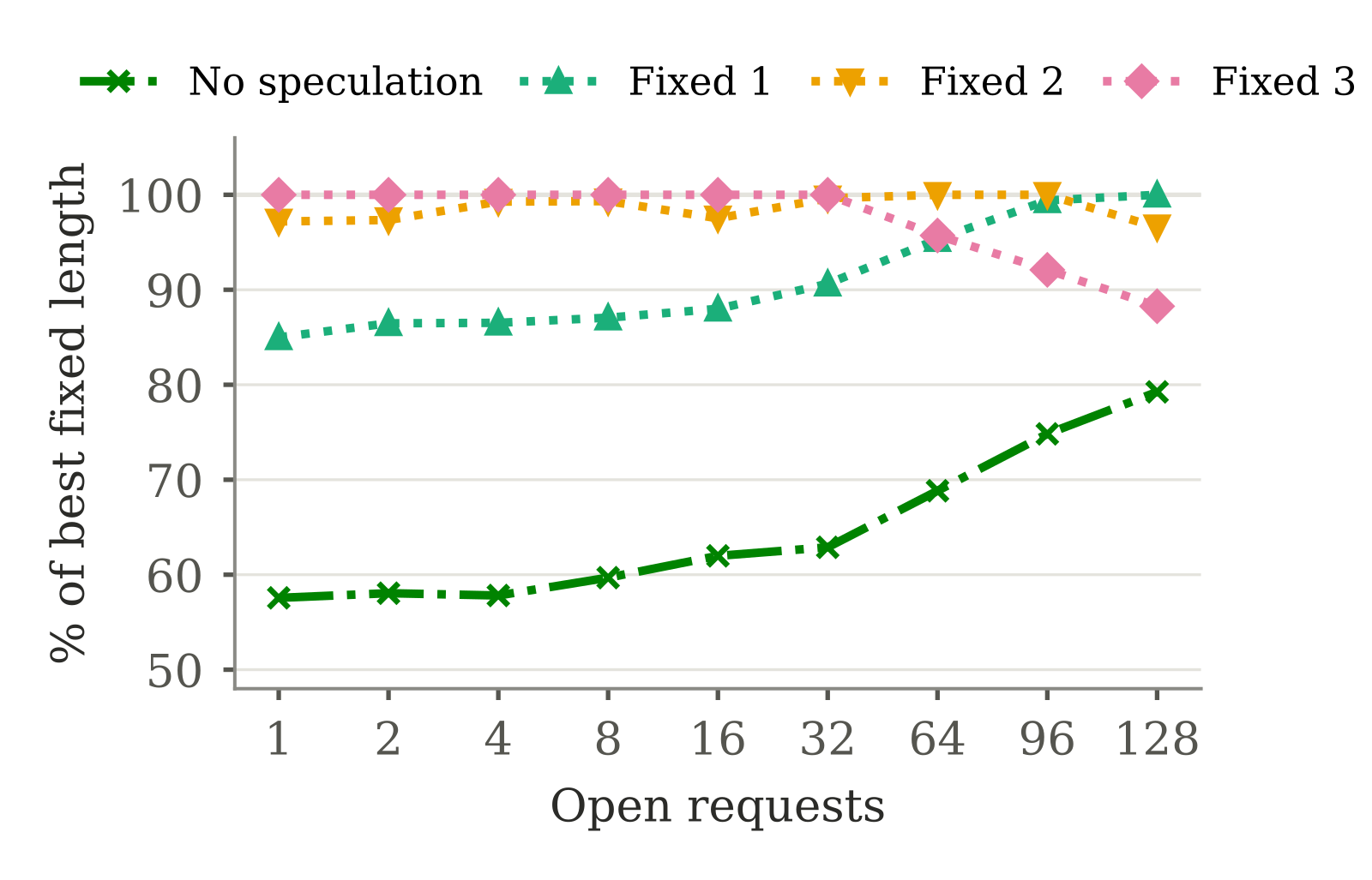
vLLM's Dynamic Speculative Decoding feature already supports looking up the length by batch size. The operator writes a table such as the documentation's example, "guess 3 up to a batch of 64, guess 1 a bit above that, and stop guessing beyond." The table is written by hand, often copied from the docs, and nothing checks it. In one user report the authors cite, turning this feature on on an H100 made serving 21% to 31% slower than no speculation at all, so an ill-fitting table can wipe out the whole gain. The best table also changes with the GPU, because older GPUs have slow steps and little spare compute: the measured table switches to length 2 at 19 requests on a T4, but only at 51 on an H100.
The overall idea: measure step time once offline, track acceptance online
The authors first separate the two quantities that set the best length. How long a step takes depends on hardware, inference engine and batch size; it is fairly stable and can be measured once offline. How often guesses are accepted depends on what the traffic contains, drifts, and has to be tracked online. TableTune follows that split:
| Part | When it runs | Input | Output |
|---|---|---|---|
| tuner | offline, once per GPU, engine, model and drafter | the real drafter and target model, 160 sample prompts | step time for each batch size and length, acceptance per position, a table in vLLM's format |
| controller | online, as a vLLM plugin | how many tokens each request guessed and kept per step, as vLLM's scheduler already records | a table rebuilt periodically, always with the tuner's step times |
Both parts maximize the same target: kept tokens per second, which the paper calls goodput.
B is the number of requests in the step, is the step time at batch size B with k guesses, and is the average number of tokens each request keeps per step. , where the 1 is the big model's own token and is the probability that the first i guesses are all accepted. Note that is not the chance that guess i alone is right: once one guess fails, all later guesses are thrown away.
A worked example you can do in your head (illustrative): with , , , guessing 1 gives and guessing 3 gives . If at some batch size a step takes 5 ms with 1 guess and 8 ms with 3, each request gets 0.34 versus about 0.31 tokens per millisecond, so this batch size should guess 1. At a smaller batch, say 4.5 ms and 6 ms, it becomes about 0.38 versus 0.42, and guessing 3 wins. The next two sections explain how each input is obtained.
The tuner: measuring every cell
The first step is timing. For each length k from 0 up to the longest allowed length K, the tuner starts vLLM with the real drafter and a one-range table, "guess k at every batch size," so the timed path is exactly the serving path, including the CUDA graph mode the server will use. For each batch size B it sends B prompts of about 32 tokens, once asking for 1 output token and once for 65; the time difference divided by 64 is one step. Each cell is the median of three repeats, every batch size up to 16 and then every 4 to 8.
Why make vLLM reject every guess while timing? If guesses were accepted, some requests would jump ahead several tokens per step and finish early, so the batch size would change in the middle of the measurement. vLLM's test mode rejects every guess: each step still does the full drafting and verification work, but all B requests advance one token per step and finish together, so the batch stays at B. The benefit of accepted guesses is added back later through . The price is that work which grows with the number of accepted tokens is never timed, and that comes back later.
The second step measures acceptance. The tuner runs the longest length K on 160 sample prompts at the serving temperature and reads two metrics vLLM already publishes: how many drafts were made, and for each position i how many kept that guess. Their ratio is . One run covers every shorter length, because a draft of length k is just the first k guesses of a draft of length K.
The last step builds the table: for each batch size it computes goodput for every length and picks the highest. To keep near-ties from splitting the table into many ranges, the tuner keeps the previous batch size's length unless another one is more than 0.5% better. The whole measurement takes about 8 minutes on an H100.
The controller: when traffic changes, the table follows
The tuner's acceptance comes from sample prompts and goes stale when the traffic changes. The controller is a vLLM plugin that changes nothing in the engine and adds no instrumentation; it uses counts the scheduler already records, how many tokens each request guessed and kept in a step. For each position it keeps two running counts: how often that position was guessed and how often it was kept. A request that guesses 3 and keeps 2 adds one to "guessed" for the first three positions and one to "kept" for the first two, because verification stops at the first wrong guess, so the kept ones are always the leading ones.
Why blend with the offline values? Right after launch there are few live counts, and dividing them directly would swing wildly. Every N steps the controller estimates:
is the tuner's value and w=2000, so the offline result counts as 2000 observations. Illustrative: with an offline and 2000 live guesses at position 2 of which 1200 were kept, the estimate is (1000+1200)/4000=0.55. After each rebuild the live counts are halved so recent traffic dominates. Only acceptance is updated; step times always come from the tuner, and the length for each batch size is picked again with the formula above. By default the choice is limited to the lengths that appear in the starting table, because the V2 runner has full CUDA graphs captured only for those.
There is a trap here. While the table runs length 1 or 0 at some batch size, nobody guesses positions 2 and 3, so the controller learns nothing about them and the table can get stuck on short lengths. The authors add two options: every 50 steps run one step at the longest length so every position keeps getting observed, and halve the prior's weight at every rebuild so old traffic fades out. When the batch size hovers near a table edge, the controller keeps the current length while the batch is within h of the edge, avoiding the back-and-forth switching that users reported as a throughput collapse.
Results: is it really better?
The main experiments run on an H100 with 1 to 128 open requests and compare how much slower each option is than the fastest fixed length at its worst load. The "best single fixed length" is chosen after the fact as the one with the smallest worst-case loss; an operator would have to benchmark every length to find it.
| Setting (H100, V2 runner) | Measured table, worst loss | Best single fixed length, worst loss |
|---|---|---|
| EAGLE-3, code prompts | 4.0% | 3.4% (length 2) |
| EAGLE-3, 4-bit AWQ target | 3.0% | 4.6% (length 2) |
| n-gram, code editing | 5.7% | 4.5% (length 5) |
| DFlash, code | 11.6% | 19.1% (length 3) |
| EAGLE-3, Spec-Bench chat | 3.1% | 3.9% (length 3) |
On a single H100 up to 128 requests, a well-chosen single length is almost as safe; the table's value is finding it without benchmarking every length. The difference shows where no single length holds up. On the mixture-of-experts model Qwen3-30B-A3B, larger batches activate more experts, so the plain step grows from 4.7 ms to 19.7 ms, while the extra cost of guessing 3 drops from 61% to 31%, so speculation keeps paying at high load. The documented table, written for dense models, switches to length 1 above 64 requests and is 17.5% slower at 96; the measured table stays within 2.9% at every load. On the older T4 and A10G, every fixed length is 7.6% to 43.6% slower at some load, while the measured tables stay within 2.3% to 5.2%.
Against existing adaptive methods, the authors reimplemented the TurboSpec and Nightjar approaches on the same engine. TurboSpec-style control picks a length every step from a fitted linear step-time model; Nightjar-style runs a separate bandit for each batch size.
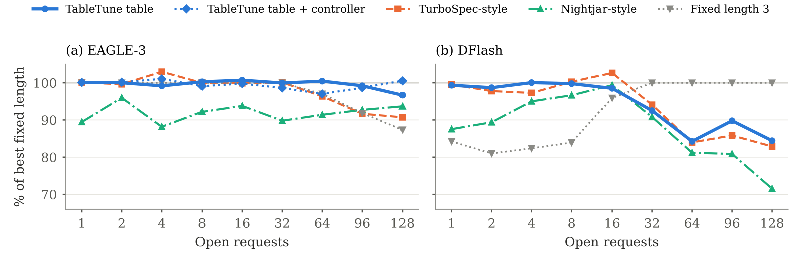
With EAGLE-3 the measured table loses at most 3.3%, TurboSpec-style 9.3% and Nightjar-style 11.8%. TurboSpec-style loses to its fit: at a batch of 80 with 3 guesses the measured step is 9.7 ms while the linear model says 8.0 ms, so it keeps guessing 3 up to a batch of about 100, whereas the measured data says to switch to 2 above 50. Step time has jumps a linear model cannot capture, so it has to be measured, not fitted. Nightjar-style is 4% to 12% slower at every load because each batch size learns on its own and keeps exploring.
The controller's repair ability was tested too. The authors deliberately start from a wrong table: the documented table with every range shrunk to a quarter, so it stops speculating above a batch of 32. On the H100 the controller raises throughput by up to 58% and reaches the measured table's level at every load, which shows that live acceptance plus offline step times is enough to fix the table. In a workload switch, DFlash runs code and then math; the stale table is 10.8% slower, and the controller rebuilds the math table within the first minute and recovers 96% of the gap, so a change in traffic does not require a new benchmark.
Finally, llm-d in its official optimized-baseline deployment: two Qwen3-32B replicas, each on two H100s with tensor parallelism, with only configuration changed. Above 256 requests the measured table is 20% to 32% faster than fixed length 3 and 7% to 25% faster than the documented table; starting from the documented table, the controller raises throughput by 9% to 29%. This shows that in a near-production multi-replica deployment, high load is where the table really matters.
Limitations as I see them
First, the gain depends heavily on the engine. vLLM's default V1 runner swaps full CUDA graphs for piecewise ones as soon as a table is set, and on the H100 every drafter that runs a model is then 30% to 43% slower with a table (n-gram, which runs no model, loses only 5.2%); only the V2 runner keeps a full graph per length and removes that loss. And this V2 nightly stalls when a table steps from length 2 to length 1, so in llm-d the authors could only deploy a table that avoids that step.
Second, the profile cannot see work that grows with accepted tokens. With DFlash at length 8, a live step takes 1.3 to 1.9 times the profiled time, so the table is up to 16% slower than fixed length 3 at batches of 34 to 87 and still 10% behind at 128 requests. The controller only updates acceptance and cannot fix such timing errors.
Third, "guess 0" in the table is not a real off switch. EAGLE-style drafters still run and keep their own KV cache at length 0, which on the H100 is 19% to 22% slower than no speculation. In the high-load range where speculation should really be off, the table does not help.
How an inference serving team could try it
- Check the engine first: with full CUDA graphs, time the best fixed length and no speculation; if setting a table makes things slower, do not use a table yet.
- Run the tuner once on your own GPU and model, put the measured table and your current hand-written table through the same load test, focus on the high-concurrency end, and judge by the worst-load loss.
- Re-measure acceptance on a week of real prompts (about 2 minutes) and see how far the table edges move; if they move noticeably, turn on the controller with both exploration and prior decay, as the authors recommend.
- If your drafter guesses many tokens at once (such as DFlash), compare live step times with the profile at a few batch sizes; if they differ a lot, do not fully trust the table.
Verdict
In one sentence: the draft-length table for speculative decoding should be measured per GPU, engine and model and updated as traffic changes; copying the docs visibly loses throughput at high load and on mixture-of-experts models.
| Dimension | Assessment |
|---|---|
| Problem importance | Medium-high. vLLM users hit it directly; the documented table is 17.5% to 25% slower on mixture-of-experts and multi-replica high load |
| Novelty | Medium. The goodput target and per-batch-size lengths come from prior work; the contribution is the measured grid and the plugin deployment |
| Evidence | Fairly strong. Three GPU types, four drafters, end-to-end llm-d, every number checkable against vLLM's metrics; but single node and short prompts only |
| Engineering cost | Low. One command, 8 to 45 minutes of profiling, a plugin with no engine changes |
| Worth trying | Yes, provided you run the V2 runner with full CUDA graphs |
How did this read for you?
Hoot made a note. Thanks for the feedback.

One tap, no sign-in; tap again to undo. Only anonymous counts are kept, never who you are.
Discussion
Add experiment details, reproduction notes or a different take. Requires a GitHub sign-in.
Loading the discussion…