Contents · 9 sections
1What problem is it solving?2The big picture3Building chains of thought: give the answer first, then filter by perplexity4Reinforcement learning: two rewards whose weights adjust themselves5Offline results: large relative gains, very low absolute values6How it is used online, and the results7Limitations as I see them8How a recommendation team could try it9Bottom line and assessmentSHARE

This is worth reading for teams doing "LLM-enhanced recommendation", where an LLM produces features for an online ranking model. Taiji does not let the LLM recommend directly. A 7B model reads the user profile and the latest 50 behaviors and reasons about "what this person will buy next"; the reasoning text is then encoded and quantized into features for the online ad ranking model. The core idea in one sentence: first build chains of thought by "knowing the answer, then reasoning backwards to a justification", filter out half by the answer's perplexity, and do supervised fine-tuning. Then align with reinforcement learning, where the reward combines "text similarity between the predicted and the true item" and "the conversion probability the online ranking model assigns to the predicted item", with the two weights adjusted automatically during training. In a one-week online A/B test, ADVV (advertiser value, a measure of advertisers' return on spend) rose 2.83% and platform revenue rose 3.30%, and long-tail users with sparse behavior gained over 5%. I find the online gains credible, but the offline metrics are very low in absolute terms, reward and evaluation use the same ranking model, and POPO (Pareto-optimal policy optimization, the automatic reward-weighting method) improves the preference metric by only 0.74% over fixed weights.
What problem is it solving?
Start with an illustrative scenario. A woman aged 31 to 40 with children has recently browsed and bought 50 items: dresses, casual pants, earrings, girls' sandals, bed sheets. Her next purchase is a bedspread. A conventional ranking model sees only a string of item IDs; an LLM can read "she is refreshing the bedding at home". The question is how to turn that understanding into features the ranking model can use and that agree with real online preferences.
LLM-enhanced recommendation usually goes through three steps: prompt the LLM directly, fine-tune it on domain data, then align it to recommendation goals with reinforcement learning. The authors see a gap in each of the last two:
| Stage | Gap |
|---|---|
| Supervised fine-tuning | Recommendation is open-ended, and one person's next purchase can have many reasonable answers, so there is no good way to judge chain-of-thought quality; checking only whether the final answer hits is too coarse |
| Reinforcement learning | Two kinds of reward are used together, a semantic reward on the LLM side and a preference reward on the recommender side, but they are usually summed with fixed weights, ignoring that one can rise as the other falls |
The big picture
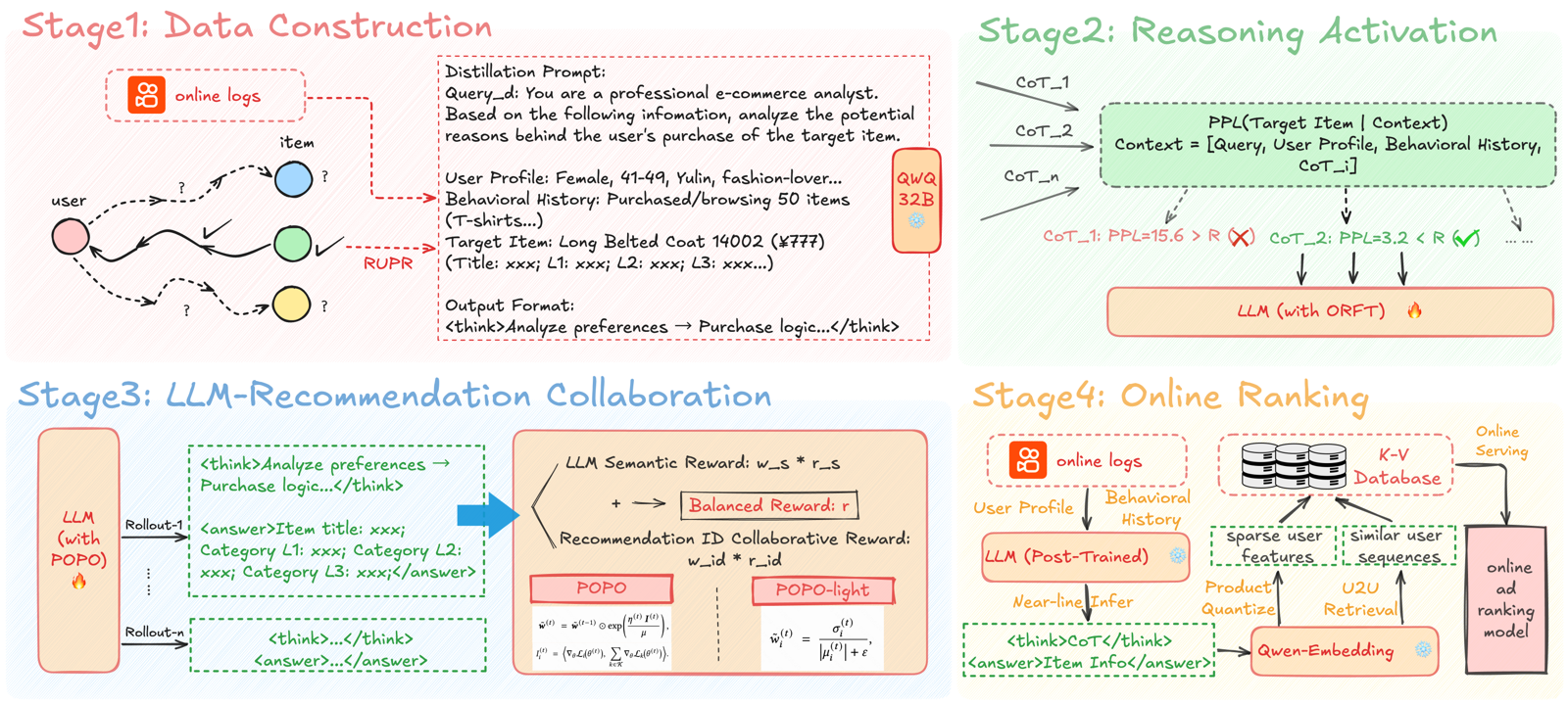
| Stage | What it does | Key numbers |
|---|---|---|
| 1. Data construction | Profile + latest 50 behaviors turned into text; with the next purchase known, QwQ-32B reasons backwards | 1.11 million user records |
| 2. Supervised fine-tuning | 3 chains of thought per prompt, keep only those below the median perplexity; fine-tune DeepSeek-R1-7B | 1 million for fine-tuning, threshold R=4.6 |
| 3. Reinforcement learning | GRPO-like training, two rewards, dynamic weights | 100K samples, 4 answers sampled per prompt |
| 4. Online ranking | Near-line inference; output encoded into sparse features and similar-user sequences | 10K test samples; serves 400 million daily active users |
Building chains of thought: give the answer first, then filter by perplexity
Stage 1 is "reverse reasoning": besides the user profile and behaviors, the prompt directly gives the item the user actually bought next and asks QwQ-32B to explain "why she would buy this". The resulting justifications at least point at the right answer, which is more reliable than letting the LLM guess and hoping it lands.
But justification quality varies, so stage 2 adds a filter. For each chain of thought, compute "the perplexity of generating the true item text, given the user information and this chain of thought". Perplexity is the exponential of the negative average per-token log probability; lower means the chain of thought steers the model toward the right answer better. As I read it, perplexity is computed by the same QwQ-32B that generated the chains, so no second model is needed. Each prompt gets 3 chains of thought, and only those below threshold R are kept, so each prompt keeps 0 to 3. R is the median perplexity on a 2.3K-sample validation set, 4.6, which roughly filters out half.
The paper gives an example. For the same user and the same target item, a bedspread, the first chain of thought infers she wants summer clothing and her next purchase may be a bag or sandals; its perplexity is 28.4 and it is rejected. The second infers she is upgrading the bedding at home and her next purchase may be a breathable, comfortable bedspread; its perplexity is 1.2 and it is kept.
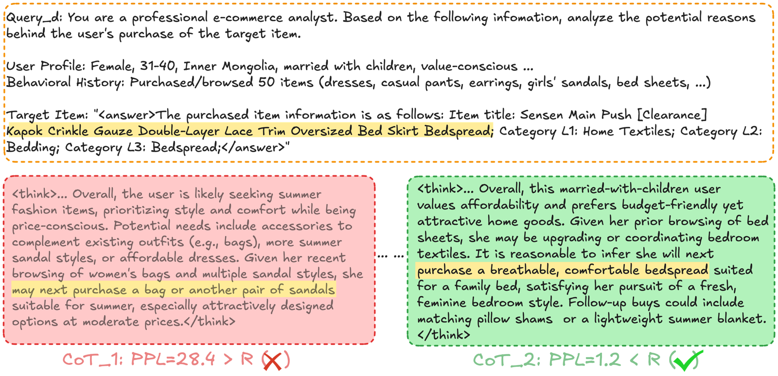
The filter is simple and useful, but note that the kept chain of thought on the right almost names "bedspread" outright. As I read it, the chain of thought is written knowing the answer, so low perplexity sometimes just means the chain of thought spelled out the answer, not that the reasoning is better. Online, the fine-tuned model has no answer to look at; what it learns is the habit of "writing a justification like this and naming a specific item".
The ablation supports reverse reasoning: compared with letting QwQ-32B reason directly from user information, level-3 category accuracy rises from 0.0185 to 0.0245, a 32% relative gain, and output-format compliance rises from 96% to 99%.
Reinforcement learning: two rewards whose weights adjust themselves
Stage 3 samples 4 answers per prompt, and each answer gets two rewards.
Semantic reward: Qwen3-Embedding-0.6B encodes the item description predicted in the model's answer and the true item description into vectors, and the reward is their cosine similarity.
ID collaborative reward: the online ad ranking model gives "user, predicted item" a probability of click and conversion, CTCVR, which is then min–max normalized. As I read it, normalization is done over the CTCVR of the same batch of answers, stretching a probability that is usually a few thousandths into the range 0 to 1, on the same scale as cosine similarity, so that weighting makes sense. To avoid calling the online service in real time during training, the authors sampled user–item pairs and their prediction scores from production and built an offline simulation environment. As I read it, the generated item description is encoded into a vector and matched only among this user's user–item pairs in the sampling pool; each of those pairs carries the ranking model's prediction score, and the score of the most similar item is taken directly as the reward. Since a most similar item always exists, there is no case of failing to match; the more off-target the description, the less the matched item resembles something the user would buy, and the lower the score naturally is.
The two rewards are combined with weights, and the advantage is computed GRPO-style: for the 4 answers to one prompt, subtract the group mean from the reward and divide by the group standard deviation. The key is how the weights are set.
POPO's approach: at each step, compute the gradient of each reward's objective separately, then take the inner product of each gradient with "the sum of both gradients". A larger inner product means optimizing along this reward also helps the other, so its weight is scaled up exponentially; a small or even negative inner product means it fights the other reward, so its weight is pushed down. Finally the two weights are normalized to sum to 1. Here is an illustrative hand example. Both weights start at 0.5. At some step the semantic reward's gradient is (1, 0), the collaborative reward's is (0.5, 0.5), and their sum is (1.5, 0.5). The semantic reward's inner product is 1.5 and the collaborative reward's is 1.0. With the ratio of step size to regularization factor set to 1, the scaled weights are 0.5×e^1.5≈2.24 and 0.5×e^1.0≈1.36, which normalize to about 0.62 and 0.38. This shows that the reward more aligned with the overall direction gets the larger weight.
The authors' theoretical guarantee is that this update can be viewed as a first-order approximation of a bi-level optimization problem whose stationary points are Pareto optimal: no policy can keep both objectives from getting worse while making at least one better.
Computing the inner product of two gradients at every step is expensive, so the authors also give POPO-light: each weight is proportional to that reward's within-group coefficient of variation, that is, standard deviation divided by the absolute mean. Here is an illustrative hand example. For one prompt's 4 answers, the semantic rewards are 0.80, 0.82, 0.78, 0.80, with mean 0.80, standard deviation about 0.014, and coefficient of variation about 0.018. The normalized collaborative rewards are 0.2, 0.6, 0.4, 0.8, with mean 0.5, standard deviation about 0.22, and coefficient of variation about 0.45. After normalization, the collaborative reward's weight is about 0.96 and the semantic reward's only about 0.04. The idea is that a reward that still separates the answers shows the model still has something to learn in that direction, so it gets more weight; a saturated reward, where the answers all look alike, has its weight lowered automatically. It uses only reward values and needs no extra backward computation.
Offline results: large relative gains, very low absolute values
The test set is 10K held-out users. Semantic metrics check whether the model's predicted level-1, level-2 and level-3 categories are correct. They also check the hit rate of the item title within the top 50 and top 100. As I read it, the model's generated item description is encoded and the 50 or 100 most similar items are taken from the candidate catalog, checking whether the true item is among them. The preference metric is CTCVR in the simulation environment.
| Metric | DeepSeek-R1-7B (not tuned) | QwQ-32B (teacher) | SFT only | + POPO-light | + POPO |
|---|---|---|---|---|---|
| Level-1 category accuracy | 0.1560 | 0.1974 | 0.2012 | 0.2347 | 0.2433 |
| Level-3 category accuracy | 0.0251 | 0.0039 | 0.0245 | 0.0307 | 0.0347 |
| Title hit rate@50 | 0.0496 | 0.0563 | 0.0449 | 0.0558 | 0.0567 |
| CTCVR | 0.003417 | 0.003675 | 0.003723 | 0.003802 | 0.003816 |
This shows the reinforcement learning step is necessary: with supervised fine-tuning alone, category accuracy rises but title hit rate falls below the untuned model; after reinforcement learning, the 7B model beats the 32B teacher on most metrics. But look at the absolute values: the best level-1 category accuracy is only 24%, and the top-50 title hit rate is under 6%.
| Metric | Fixed weights 0.5/0.5 | POPO-light | POPO |
|---|---|---|---|
| Level-1 category accuracy | 0.2180 | 0.2347 | 0.2433 |
| Level-3 category accuracy | 0.0269 | 0.0307 | 0.0347 |
| Title hit rate@100 | 0.0698 | 0.0762 | 0.0720 |
| CTCVR | 0.003788 | 0.003802 | 0.003816 |
Compared with fixed weights, POPO raises level-3 category accuracy by 29% relative, but CTCVR by only 0.74%. This means dynamic weighting mainly lifts the semantic side, with little gain on the preference side. POPO-light adds almost no overhead and even beats full POPO on title hit rate@100, so using it when GPU budget is tight is a reasonable choice.
How it is used online, and the results
The trained model runs near-line inference: for each user it generates a chain of thought and predicted item information, which Qwen-Embedding-0.6B encodes into a vector used in two ways.
| Use | How | ADVV | Revenue |
|---|---|---|---|
| Intra-user features | The vector is turned into sparse ID features by product quantization | +1.06% | +1.35% |
| Cross-user sequences | Find the 1 most similar user by cosine similarity of vectors, and take their latest 100 behaviors as an extra sequence feature | +1.77% | +1.95% |
| Total | +2.83% | +3.30% | |
| Total (long-tail users) | +5.26% | +5.32% |
The A/B test gave 10% of traffic to each arm and ran for one week. The "Total" row is exactly the sum of the first two rows; as I read it, the two paths are increments measured separately. Cross-user sequences contribute more than intra-user features, which is interesting: the most useful outlet for the LLM's understanding may be helping users with few behaviors find a behavior-rich "similar user" to borrow data from. The doubled gain for long-tail users fits this explanation.
Limitations as I see them
First, reward and evaluation use the same model. The collaborative reward in reinforcement learning comes from the CTCVR given by the online ranking model, and the offline preference metric is the same simulated CTCVR. So part of CTCVR's rise from 0.003417 to 0.003816 is "learning to please this ranking model", and it cannot be taken directly as evidence of more accurate user preferences. The online A/B test is the real check.
Second, the gain from dynamic weighting on the preference side is small. Compared with fixed 0.5/0.5 weights, POPO adds only 0.74% CTCVR. The Pareto-optimality guarantee covers stationary points of full POPO, while POPO-light, the more practical choice in industry, is a heuristic based on the coefficient of variation and falls outside that guarantee. The online table splits the two feature uses, not the two weighting methods, so POPO's own online contribution cannot be read from it.
Third, the bar for reproduction is high. Training uses 3 machines with 8 A800 GPUs each, and prompts run up to 13,000 tokens. The paper's learning rates are 1e-7 for supervised fine-tuning and 2e-5 for reinforcement learning; the former is roughly two orders of magnitude below common settings, so it needs retuning when reproducing. On top of that, reverse reasoning may write the answer into the chain of thought (see the example above), so the filtering threshold is best checked on your own data.
How a recommendation team could try it
- Start without training: have an open-source reasoning model read the user profile and recent behaviors and produce "what they may buy next", encode it, find the 1 most similar user, and add that user's behavior sequence as an extra feature to the ranking model; check offline AUC, especially for users with few behaviors.
- If that works, build chains of thought: reason backwards from the true next purchase, generate several, and filter half by perplexity; at the same time, sample how many kept chains of thought spell out the answer directly.
- For reinforcement learning, first run a version with fixed weights, then switch to POPO-light, and compare each reward's curve rather than just the weighted total.
- Online, A/B test "intra-user features" and "cross-user sequences" separately to see which path the gain comes from.
Bottom line and assessment
The most useful takeaway is that one of the most useful outlets for an LLM's understanding of users is helping sparse users find similar users, and a rule like POPO-light's "give more weight to whichever reward still discriminates" costs almost nothing and can be dropped straight into a GRPO training loop.
| Dimension | Assessment |
|---|---|
| Importance of the problem | High. LLM-enhanced recommendation is widely used in industry, and weighting multiple rewards is a common problem |
| Novelty of the method | Medium. Reverse reasoning and perplexity filtering combine existing work; POPO borrows dynamic weighting from multi-domain optimization |
| Experimental evidence | Medium. The online A/B is large with clear gains; the offline reward and evaluation share a source, and POPO's online contribution is not separated out |
| Engineering cost | High. Near-line 7B inference covering 400 million daily active users, plus K-V storage and similar-user retrieval |
| Worth trying? | Yes, starting with the cross-user sequence path |
| Where it fits | Advertising and e-commerce recommendation, especially businesses with a large share of long-tail users with sparse behavior |
How did this read for you?
Hoot made a note. Thanks for the feedback.

One tap, no sign-in; tap again to undo. Only anonymous counts are kept, never who you are.
Discussion
Add experiment details, reproduction notes or a different take. Requires a GitHub sign-in.
Loading the discussion…