Contents · 7 sections
1Where current unified backbones compress the history2Fine interactions stay inside a group; across groups, only narrow paths3Walkthrough: how a history of 1,536 events goes through three layers4How quality and cost move together on the public benchmark5Longer and more skewed histories, and the online bill6What this means for people building unified recommendation backbones7LimitationsSHARE

You want to read 1,536 behaviors one by one, but compute grows with the square: how TokenFormer V2 splits resolution from interaction density
You need to predict whether a user will convert after clicking an ad. This person has left a long record across four behavior domains, and the model looks at up to the most recent 1,536 events. A few nearby actions, taken together, reveal an intent that no single event can state on its own. You want the model to read each record in the context of neighboring events and the current request, then decide which ones help this prediction.
But the serving budget is tight. Dense self-attention over all 1,536 events grows with the square of the length. To save compute, recent unified recommendation backbones often compress the history into a shorter summary first. OneTrans puts fields and behaviors into one causal stream; deeper layers keep fewer behavior representations in the computation. HyFormer and MixFormer use feature-derived queries to pool history into a compact state, and later feature interaction runs on that summary. At prediction time, the model can no longer line up with every encoded behavior.
This paper builds a unified backbone for industrial recommendation, and the problem it takes on is this dilemma between resolution and compute: modeling a long history in fine detail is too expensive, and compressing it into a summary limits the evidence that prediction can use. It proposes TokenFormer V2, which separates representation resolution from interaction density. Every retained behavior keeps its own token throughout encoding, fine interactions happen only inside a group, two narrow paths handle communication across groups, and the final prediction can still read every encoded behavior directly. On the public evaluation of the Tencent Advertising Algorithm Competition 2026 (TAAC 2026), relative to the strongest baseline, MixFormer, its AUC rises by 0.10 percentage points, and its forward FLOPs are only 19.5% of MixFormer's. In live WeChat Channels ad traffic, relative to the production model, GMV rises by a statistically significant 2.33%.
Separating representation resolution from interaction density means fine-grained history does not have to be shortened first to fit the budget; the online 2.33% GMV lift is against the production model.
Where current unified backbones compress the history
A unified recommendation backbone has to do two jobs in one model: read interests from a behavior sequence, and cross features among fields that are not ordered in time, such as user, candidate, and request. The authors' earlier TokenFormer already puts fields, behaviors, and the target into one causal stream, but the shallow layers still use full attention, so the quadratic cost remains. OneTrans, HyFormer, and MixFormer trade compression for speed: they either reduce how many behavior representations deeper layers can still see, or first pool the history into a short query state.
Return to this history of at most 1,536 events. If a few nearby actions have to be read together to become clear, and the compression happens too early, later layers can never get back to those events' individual representations. What TokenFormer V2 wants to keep is exactly this individual evidence, still directly readable. It calls this property full resolution: at prediction time, the model can still attend directly to every encoded event.
Fine interactions stay inside a group; across groups, only narrow paths
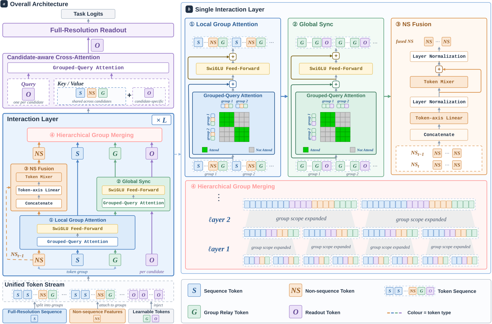
To keep every behavior, without computing attention between every pair of tokens, the model has to specify who can interact with whom directly. TokenFormer V2 cuts the behavior sequence into consecutive groups, and assigns each group a share of non-sequential tokens (NS, holding user, candidate, and request fields) plus a set of learned group-relay tokens. Inside a group, it runs dense Local Group Attention: each behavior representation takes in neighboring events and field context, and the field tokens are also updated by this slice of history.
Across groups, the model does not run another large-scale attention. NS Fusion concatenates the field representations that entered this layer with the versions just updated inside each group. It applies a learned linear mix along the token axis, then adds a residual from a RankMixer-style parameter-free channel-block permutation. It then splits the result back to the groups, so that every group in the next layer can use field context filled in by other slices. RankMixer was originally used for field-token mixing and per-token feed-forward. Global Sync lets group-relay tokens and a small number of readout tokens exchange information in a shared space: the relays bring global context back to each group, and the readout tokens accumulate queries for the final prediction.
As depth increases, neighboring groups are merged. The paper gives a small example: two groups of 4 behaviors each merge into one group of 8 behaviors. Each behavior remains its own representation; it simply sees more neighbors directly. Merging widens the interaction range; it does not pool the 8 events into 1 summary. The token inventory stays fixed across the whole stack.
The last step is Full-Resolution Readout. The readout tokens serve as queries, run candidate-aware cross-attention over all encoded behaviors, fields, relays, and readout tokens, and are then mapped to each task's prediction. The prediction head still faces that full history, which is still there, not a summary that has already been shortened.
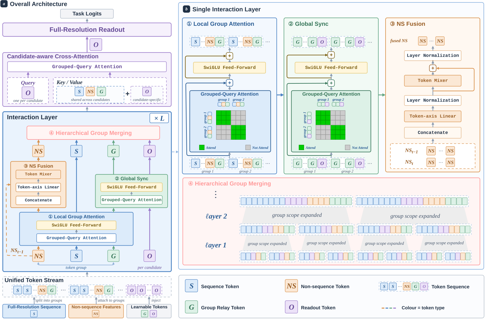
If you switch to a simpler design, the bill splits immediately. Full attention throughout would keep the resolution, but the cost grows with the square, and the authors' earlier TokenFormer already paid that bill in its shallow layers. Compressing into a summary first saves compute, but the prediction head can no longer line up with every event. TokenFormer V2 keeps fine interactions inside each group, and hands cross-group communication to a much smaller number of context tokens. When group size is bounded, local attention is linear in the total number of tokens; if the number of groups is written as b, this term is about 1/b of full attention under balanced grouping. Hoot says
The article already walks the default setup: 1,536 history events through three layers. This walkthrough only pursues a point that walk did not unpack: when history gets longer, when local attention grows linearly, and when it grows with the square. The same illustrative numbers are used below, doubling history from 1,536 to 3,072, and comparing only the local-attention term.
default 16 groups × 96 positions → if the group count stays 16, each group has 192 and local attention is about 4× → if group size stays 96, there are 32 groups and about 2× → the long-history experiment does not state its grouping schedule, so it cannot tell which knob was turned
- default first layer → 16 groups of 96 positionsUnder the paper's default setup, at most 1,536 behaviors are split into 16 groups in the first layer, and each group covers 96 positions. Local attention is computed only inside a group.1536 / 16 = 96
- fixed 16 groups + doubled history → about 4× local attentionIllustrative: if history grows to 3,072 events and the group count stays 16, each group becomes 192 positions. The in-group cost grows with the square of the length, so 192² / 96² = 4, and across 16 groups this local-attention term is about 4 times the original.16 × 192² is 4 times 16 × 96²
- group size stays 96 + doubled history → about 2× local attentionThe same illustrative numbers: if each group is still limited to 96 positions, the group count has to rise from 16 to 32, each group's cost stays the same, and local attention is about twice the original. That is what the article means by “when group size is bounded, local attention is linear in the total number of tokens.”32 × 96² is 2 times 16 × 96²
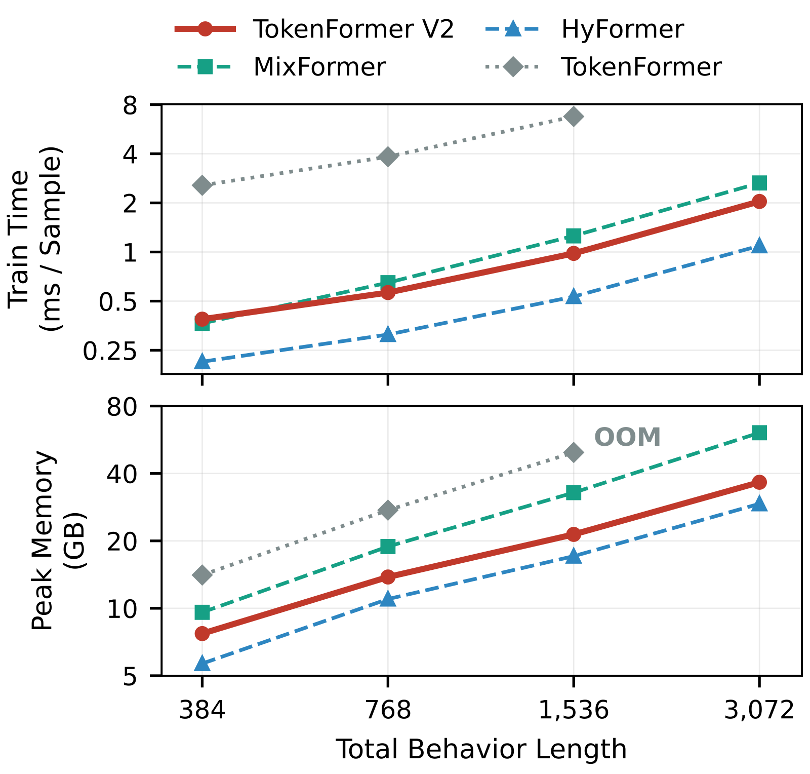
- long-history timings → cannot confirm the grouping scheduleWhen the paper scales history to 3,072 events, it reports training time and memory, but it does not say whether that run kept the group count fixed or kept group size bounded. The growth curves in Figure 3 therefore cannot be used to infer which knob was turned.the article does not give the group count at 3,072 events
Full attention throughout would grow with the square. The calculation here is only the local-attention term; it does not include NS Fusion, Global Sync, or the feed-forward. Linear growth holds when group size is bounded, not merely because every behavior keeps its own token.
Source
Paper §3.4: local attention is linear in the total token count N when group size is bounded; under balanced grouping it is O(d N^2 / b). §4.1 default: at most 1,536 events, group schedule 16→8→4, first-layer span 96. §4.3–4.4 scale history to 3,072 but do not state the grouping schedule used there. The doubled-history 16×192 versus 32×96 comparison is illustrative.Walkthrough: how a history of 1,536 events goes through three layers
The next stretch is a worked example of the default TAAC setup in Section 4.1 of the paper; every number comes from the paper, not from a separately made illustration. Four domains are concatenated into a sequence of at most 1,536 events. The model has three layers, width 192, and a grouping schedule of 16→8→4. There are also 64 NS tokens, 32 group-relay tokens, and 4 readout tokens.
Step one is grouping. The first layer has 16 groups, and each group covers 96 positions. The 64 NS tokens and 32 relays are split evenly across groups, so each group gets 4 NS tokens and 2 relays. If all 96 positions have a behavior, the group has 96+4+2=102 tokens in total, and they attend to each other bidirectionally. So after this step, each behavior representation already includes neighboring events and field context, but it still cannot see the events themselves outside the group.
Step two is communication across groups. The behavior tokens keep their locally encoded results; they are not replaced by a single group summary. NS Fusion first concatenates the 64 NS tokens that entered this layer with the 64 versions updated inside the groups, then applies a learned linear map along the token axis, and obtains 64 NS tokens again. This way, each output token has mixed in the field evidence just updated in the groups. It then applies a RankMixer-style parameter-free permutation as a residual mix: the 64×192 representation is reshaped to 64×64×3, the first two axes are swapped, and it is reshaped back to 64×192, which is equivalent to transposing channel blocks across tokens. These 64 updated NS tokens are split back to the groups in the next layer, so the field context each group receives already carries evidence from other slices. Global Sync lets the 32 relays plus 4 readout tokens, 36 in total, run self-attention in the shared space: the relays bring global context back to each group, and the readout tokens keep accumulating queries for prediction.
Step three is hierarchical merging. The second layer merges neighboring groups into 8 groups, and the range of direct interaction in each group grows from 96 positions to 192. This is the same as the earlier example of 4 events becoming 8: the 192 events are still 192 tokens, not pooled into one summary; they simply see more neighbors directly. This shows that merging widens the interaction range, while individual behaviors are still kept separately.
Step four: the third layer merges again into 4 groups, each spanning 384 positions. Cross-group communication has already happened at every layer, so the model does not have to wait until everything is collected into one group before distant information arrives. At this point, at most 1,536 behaviors are still 1,536 behaviors.
Step five is Full-Resolution Readout. The 4 readout tokens serve as queries, run cross-attention over all encoded behaviors as well as the NS, relay, and readout tokens, and are then mapped to the conversion prediction. The prediction head still looks directly at every encoded behavior.
If the first layer put about 1,536+64+32 tokens together for attention, the compute would grow with the square; after splitting into 16 groups, local attention is about 1/16 of that. This is what "the resolution remains, the interactions get sparser" means on the bill.
To see whether every part of this split is useful, look at what happens when one piece is removed. The authors drop one component at a time, retrain on the full training data, and obtain Table 4. The table also includes an attention-output gate, applied to the attention outputs of local attention and of Global Sync.
| Variant | Test AUC | Change (percentage points) |
|---|---|---|
| TokenFormer V2 | 0.8221 | — |
| Fixed 16 groups, no merging | 0.8219 | -0.02 |
| No NS tokens inside a group | 0.8212 | -0.09 |
| Without NS Fusion | 0.8217 | -0.04 |
| Without Global Sync | 0.8209 | -0.12 |
| Without the attention-output gate | 0.8218 | -0.03 |
(Numbers from paper Table 4)
This shows two things that matter most: local encoding needs field context, and the groups need to be connected. Removing Global Sync drops 0.12 percentage points, and dropping NS tokens inside a group drops 0.09, both much larger than the 0.02 from not merging. The ablation can show that each component contributes; it cannot show that the merge schedule itself contributes the most, because the fixed 16-group variant stays at almost the same level.
How quality and cost move together on the public benchmark
TAAC 2026 provides 47.10 million conversion-labeled impressions, with four behavior domains labeled A through D. The test set is 12.30 million later impressions, and its users do not overlap with the training set. All models share the input features, the data pipeline, a 64-dimensional embedding table, and the prediction head, and their dense parameters all sit around 11 million. The comparison is on test AUC, log loss, and forward FLOPs per example.
| Model | Test AUC | Forward GFLOPs |
|---|---|---|
| Transformer | 0.8168 | 32.59 |
| TokenFormer | 0.8198 | 28.52 |
| HyFormer | 0.8204 | 3.13 |
| MixFormer | 0.8211 | 19.75 |
| TokenFormer V2 | 0.8221 | 3.86 |
(Numbers from paper Table 2)
Relative to the strongest baseline, MixFormer, TokenFormer V2 raises AUC by 0.10 percentage points, lowers log loss by 0.40%, and uses only 19.5% of MixFormer's forward FLOPs. Under the same setup, inference is 2.6 times faster, and training throughput is 21% higher. This shows that the lead is not bought by piling on more compute: the cost drops sharply, and the ranking still gets better.
Relative to the authors' earlier TokenFormer, AUC rises by 0.23 percentage points, FLOPs fall by 7.4 times, and amortized inference latency falls by 6.9 times. This shows that replacing shallow full attention with the grouped layout can keep the resolution and still bring the cost down.
Relative to a standard Transformer, AUC rises by 0.53 percentage points, and FLOPs are 8.4 times lower. Compared with the cheaper HyFormer, V2 is a little more expensive, 3.86 versus 3.13 GFLOPs, but AUC is still 0.17 percentage points higher. This shows that keeping every behavior in full can still land in a compute range close to a query-pooling model, while ranking higher. They train for the same epoch and validate every 4k steps; V2 leads at every measured checkpoint. At the 4k-step mark, it is already ahead of TokenFormer, HyFormer, and MixFormer by 0.20, 0.27, and 0.25 percentage points, respectively.
Longer and more skewed histories, and the online bill
The four domains are scaled together to lengths from 384 to 3,072, and training time and peak memory are measured on one H20, with batch size 256 and the history fully filled. When history is scaled 8 times, TokenFormer V2's training time grows to 5.3 times and memory to 4.7 times, very close to HyFormer's 5.1 times. At 3,072 events, it trains 23% faster than MixFormer and uses 40% less memory. On the lengths it can finish, TokenFormer takes 6.6 to 6.9 times as long, and at the maximum length it exceeds 96 GB of memory. This shows that keeping every behavior does not necessarily return to the scaling of full attention.
After the models are retrained at a history of 3,072 events, TokenFormer V2 still leads: it is 0.09 percentage points above MixFormer, with 4.4 times fewer FLOPs. Its default 1,536-event setup already beats every compared model trained with the doubled history. Under the default budget it already beats the compared models after they double their history, so it does not have to double the input first to hold up.
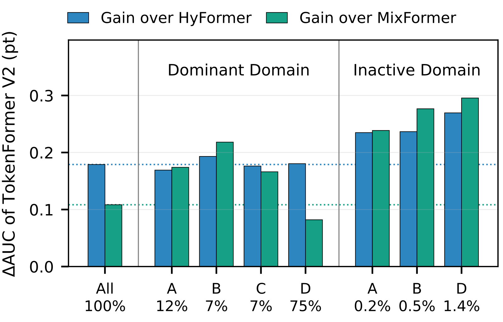
Unbalanced users are not just carried along by the majority domain. Domain D dominates about three-quarters of test impressions, and users dominated by A through C are used to check whether the model can still hit the mark outside the majority domain. Relative to MixFormer, the gain on D-dominated users is about 0.08 percentage points, 0.17 to 0.22 for users dominated by A through C, and 0.24 to 0.30 for users who have no events at all in some domain. Relative to HyFormer, the gain on users with a missing domain is 0.24 to 0.27. This shows that the overall 0.10 percentage points is larger on users outside the majority domain.
The industrial comparison is on the post-click conversion rate (pCVR) ranking stage of WeChat Channels ads. The models' dense parameters are first aligned to about 1 billion on historical production logs, and the standard setup also shares the same input features. In production, TokenFormer V2 encodes newer and older behaviors on different branches, assigns deeper encoding to more recent activity, then connects the branches with NS Fusion and Global Sync, and the final readout can still see every encoded behavior.
MixFormer-1B has an overall AUC of 0.8004 and 15.3 forward GFLOPs. TokenFormer V2-1B is the only challenger that beats it, with overall AUC 0.0572 percentage points higher, but the cost is 70.2 GFLOPs, more expensive than MixFormer. This shows that on production logs at about a billion parameters, the accuracy advantage remains, but the cheaper-compute comparison from TAAC cannot be reused. After the sparse input features provided by a conventional model such as DCN-V2 are removed, the variant called TokenFormer V2-1B* cuts the cost from 70.2 to 23.1 GFLOPs, a drop of 67.1%, and the overall AUC gain goes further to 0.0712 percentage points. The billion-parameter versions of HyFormer, OneTrans, and TokenFormer all have lower overall AUC than MixFormer.
The online A/B comparison is against the production model, not against MixFormer in Table 5. The two groups share the same features, training sample stream, bidding strategy, and serving budget; only the ranking backbone is changed. TokenFormer V2 raises GMV by a statistically significant 2.33%, and raises online AUC by 0.16%. This shows that the extra offline ranking quality became a business lift in live traffic; it does not show that 2.33% is also a number relative to MixFormer.
What this means for people building unified recommendation backbones
First check whether your unified backbone compresses long history into a summary the prediction head can no longer read; if it does, TokenFormer V2 offers an organization already tested online: keep the resolution, and control interactions by group.
The grouping schedule and the two narrow paths are knobs you can move over and try. On TAAC, the 16→8→4 schedule widens the local span from 96 to 384, but the 1,536 behaviors remain throughout. If you care more about serving cost, do not take that 19.5% FLOPs figure from TAAC as the bill in a billion-parameter production setting, because on WeChat Channels logs, standard TokenFormer V2-1B is more expensive than MixFormer-1B, and the variant that actually brings the cost down is the one that drops those sparse auxiliary features. You can also split offline metrics by dominant domain and missing domain first; in this paper, the larger gains appear outside the majority domain.
Limitations
The 19.5% forward-FLOPs comparison belongs only to the TAAC setting with about 11 million dense parameters, against MixFormer. On WeChat Channels logs at about 1 billion parameters, standard TokenFormer V2-1B costs 70.2 GFLOPs, higher than MixFormer-1B at 15.3; even the simplified-input V2-1B* is still 23.1, so it does not fall below the other model.
The online 2.33% GMV lift is against the production model. The paper does not name this production model, and it does not compare the same online experiment directly with MixFormer.
The ablation retrains after dropping one component at a time; it can show that each block contributes, but it cannot show how they amplify one another. Fixing 16 groups drops only 0.02 percentage points, and the merge schedule is the weakest item in this table. The public evaluation is also run only on this one advertising dataset, TAAC 2026.
How did this read for you?
Hoot made a note. Thanks for the feedback.

One tap, no sign-in; tap again to undo. Only anonymous counts are kept, never who you are.
Discussion
Add experiment details, reproduction notes or a different take. Requires a GitHub sign-in.
Loading the discussion…