Contents · 11 sections
1What problem does UCGRec solve2First, what the user-centric graph is3How the three signals are picked4How the graph enters the LLM5Experimental setup: HR@1 with 20 candidates6Main results7Ablations: which design actually matters8Problems in the evidence9Cost10How to try it in your own system11Conclusion and assessmentSHARE

UCGRec is about LLM-based sequential recommendation: give LLaMA 2-7B a user's history and 20 candidates, and have it write out the next movie the user will watch, artist they will play or toy they will buy. Its contribution is to filter three kinds of user signal separately and then join them into a small graph that belongs to this one user, encode it with a GNN and put the result into the prompt. The three signals are long-term interests that are semantically consistent, the most recent few actions, and collaborative paths sampled by random walks that start from each item in this user's history and run over a global graph built from all users' transitions. In the ablations the design with the largest payoff is "use only this small graph, not the full collaborative graph": on LastFM, HR@1 rises from 0.4391 to 0.5447 (Table 4). In the main experiment the average HR@1 over four datasets is 0.5252, above LLaRA's 0.4895 (Table 1). My judgment: the idea is clear and worth borrowing, but the main evaluation is 1-out-of-20 (full-catalogue retrieval is tested on only two datasets), several appendix tables disagree with the main table, and the written cold-start conclusion claims more than the numbers in its table.
What problem does UCGRec solve
LLM recommendation writes the user's history as a text prompt and has the model generate the next item. The authors see three flaws in this. The history mixes in misclicks and casual exploration, and feeding all of it in disturbs the model's judgment. Earlier methods usually use only one of long-term interest, short-term interest and the collaborative signal from similar users. Even when all three are given, listing them separately in the prompt does not let the model see how they relate, while also costing more tokens.
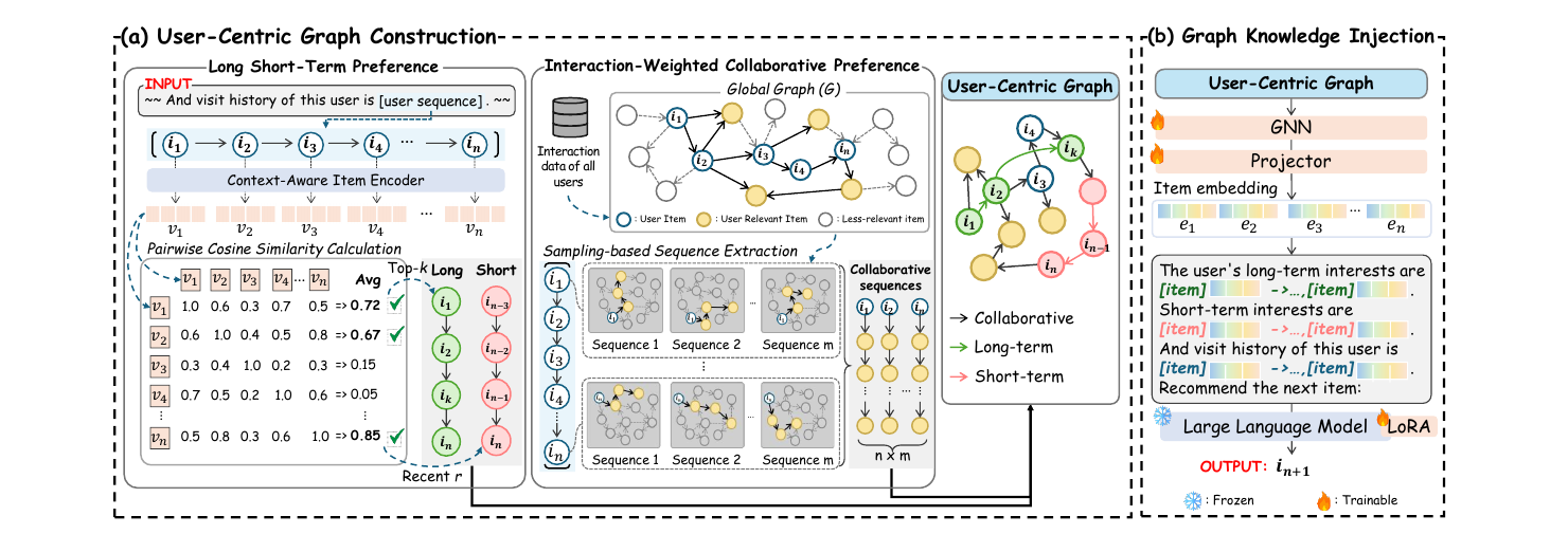
UCGRec does one thing for each of these points: it uses semantic similarity of item descriptions to pick out "stable interests", uses a weighted graph walk to take only the collaborative paths relevant to this user, and then merges those paths with the user's own sequence into one graph. A GNN reads this graph; the item embeddings it produces are mapped into the LLM's token space by an MLP projector and placed right after the matching item titles in the prompt. The GNN, the projector and the LLM's LoRA are trained together end to end (Section 3.2).
First, what the user-centric graph is
The key to this paper is keeping two graphs apart.
The global graph is built from every user's behaviour: each item is a node, and whenever some user clicks A and then immediately B, a directed edge goes from A to B, with a weight equal to how often that order appears across the whole dataset (Section 3.1). On LastFM this graph has 4,606 nodes, that is, every artist (Table 11).
The user-centric graph is a small graph built separately for each user. Its nodes come from four places: the user's own last 10 actions; the long-term sequence picked from them; the short-term sequence made of the last r items; and the collaborative paths walked on the global graph starting from each item in the user's history. The linking rule is that adjacent items within each sequence get an edge. The user's history and the short-term sequence are linked in time order, the long-term sequence in its similarity-ranked order (the pink and green edges in Figure 1), and the collaborative paths in walk order (black edges). These sequences share the same item nodes, and every collaborative path starts at an item from the user's history, so together they form one graph. When the same edge appears in several sequences, its weights add up. On LastFM this small graph averages 192.22 nodes (Table 11).
The authors' claim fits in one sentence: collaborative signal helps, but only the small piece relevant to this user should be taken, and it should reach the LLM as graph structure rather than flat text. Almost every later ablation tests this sentence.
How the three signals are picked
Long-term interest is picked by semantic consistency. An item title carries too little information, so the authors first have LLaMA 3-8B write a description from the title (genre, plot summary and so on), then encode the description into a vector with Sentence-BERT. For each item in the user's history they compute its average cosine similarity to all items in the history and keep the k highest-scoring items as the long-term sequence (Equations 1 and 2). Intuitively, if a user watched seven comedies and two horror films, the comedies will have high average similarity, while a documentary opened by chance scores lowest and is dropped.
Short-term interest is the simplest: the last r items (Equation 3).
Collaborative signal comes from walking on the global graph. From each item in the user's history, a walk of z steps yields one path, repeated m times per starting item. At each step the walk moves to the neighbour with the largest edge weight with probability α, and to a random neighbour with probability 1−α (Equation 4). α is 0.6; the authors explain that this leaves room for randomness, so paths are not always pulled along by a few popular transitions. Defaults are k=r=3, m=6 and z=10 (Appendix A.5).
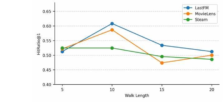
The walk length z decides whether this small graph degenerates into the global graph. Figure 3 plots HR@1 for different z: LastFM and MovieLens both peak at z=10 and decline for longer walks; Steam is roughly flat up to z=10 and also declines afterwards. The authors explain that the further the walk goes, the more the paths resemble the global graph and the more unrelated users get mixed in (Appendix A.7), which suggests that limiting the walk range and reducing unrelated information helps preserve the target user's signal, in the same direction as the Table 4 result. The experiment changes range and relevance together, so it does not isolate the effect of graph size itself.
How the graph enters the LLM
Node vectors are initialised with pretrained SASRec item embeddings (64 dimensions). The GNN aggregates neighbours by edge weight: 1-hop neighbours on LastFM and 4-hop on the other three datasets (Appendix A.5). The GNN's output vectors are mapped to LLaMA 2-7B's token dimension by the MLP projector.
The prompt looks like this (Appendix Table 14): "This user's long-term interests are [item][vector] → … ; short-term interests are [item][vector] → … ; the visit history is [item][vector] → … ; choose the next movie from the following 20." In the long-term, short-term and history sequences, every item title is followed by one vector token computed from the user-centric graph through the GNN and the projector (Section 3). Appendix Table 14 uses colour to separate two kinds of vectors. The LLaRA prompt has grey pretrained vectors carrying only simple collaborative information, while the three sequences in the UCGRec prompt have blue vectors that integrate user-centric graph knowledge. During training the LLM body is frozen and only LoRA (rank 8), the GNN and the projector are updated, for 37.1M trainable parameters, only slightly more than LLaRA's 37.0M (Table 11).
The difference from LLaRA needs to be stated precisely. LLaRA also appends a pretrained ID embedding after each item title, and these pretrained ID vectors carry indirect collaborative information, but they are not aggregated over a graph built around the target user; UCGRec's vector has been aggregated by the GNN over neighbours in the user-centric graph, so the same item gets a different vector in different users' prompts.
Experimental setup: HR@1 with 20 candidates
The experiments use four public datasets, MovieLens, Steam, LastFM and Amazon Toys, all small; the largest, Toys, has 97,682 users (Appendix Table 9). Preprocessing follows LLaRA and keeps only each user's last 10 actions (Appendix A.3), so "long-term interest" here means picking 3 out of 10 items, which is a different thing from the industrial long sequences of thousands of actions.
The evaluation protocol decides how to read the numbers that follow. Each test example gives the model 20 candidates: the one true next item plus 19 random items the user never interacted with (Appendix A.5). Only 1 of the 20 candidates is correct, so random guessing would score an expected HR@1 of 0.05. ValidRatio is the fraction of model outputs that match some item in the candidate list; the authors consider HR@1 trustworthy only when it is above 0.95 (Section 4.3), because an output outside the candidates is not a recommendation at all. Temperature is 0 and results are averaged over 5 random seeds.
Baselines fall into three groups: traditional sequential models GRU4Rec, SASRec and GCE-GNN; zero-shot LLMs, LLaMA 2-7B and GPT-4o; and fine-tuned LLM recommenders, where TALLRec and LLaRA fine-tune the LLM with LoRA while A-LLMRec and LLM-SRec freeze the LLM and train only an encoder and projector (Section 4.2).
Main results
| Method | LastFM | MovieLens | Steam | Toys | Average |
|---|---|---|---|---|---|
| SASRec | 0.2233 | 0.3444 | 0.4010 | 0.4157 | 0.3457 |
| GCE-GNN | 0.3181 | 0.4295 | 0.4484 | 0.2405 | 0.3591 |
| GPT-4o (zero-shot) | 0.3443 | 0.2151 | 0.3653 | 0.4127 | 0.3344 |
| TALLRec | 0.4974 | 0.4695 | 0.4356 | 0.4843 | 0.4717 |
| LLaRA | 0.4803 | 0.4758 | 0.4886 | 0.5133 | 0.4895 |
| LLM-SRec | 0.3590 | 0.4211 | 0.4862 | 0.3749 | 0.4103 |
| UCGRec | 0.5447 | 0.4949 | 0.5040 | 0.5574 | 0.5252 |
All values are HR@1 from Table 1. UCGRec ranks first on all four datasets, and on average it is 11.3% above TALLRec and 7.3% above LLaRA (relative gains, Section 5.1); the authors report the differences as significant at p<0.05. Its ValidRatio is above 0.97 on all four datasets, meaning the model almost always outputs an item from the candidates, so HR@1 can be taken at face value.
Two details of this table matter. The closest competitor is LLaRA, which happens to be the "append pretrained item vectors to the prompt" approach, so the 7.3% gap is a more useful reference than the comparison against GPT-4o. It is still the gain of the full UCGRec system over LLaRA, and the two also differ in long- and short-term preference extraction and in the prompt, so it cannot all be attributed to graph aggregation. The other detail is Steam: UCGRec 0.5040 against LLaRA 0.4886, a gap of only 0.0154, the smallest of the four datasets.
Ablations: which design actually matters
The paper runs three groups of ablations; the table below puts them together, all values HR@1:
| Comparison | LastFM | MovieLens | Steam | Toys | Source |
|---|---|---|---|---|---|
| Long-term signal only | 0.5146 | 0.4750 | 0.4962 | 0.5121 | Table 2 |
| Short-term signal only | 0.5328 | 0.4215 | 0.4829 | 0.5497 | Table 2 |
| Collaborative signal only | 0.5344 | 0.4586 | 0.4675 | 0.5504 | Table 2 |
| Long-term by random sampling | 0.4869 | 0.4745 | 0.5008 | 0.5493 | Table 3 |
| Long-term as the full history | 0.5146 | 0.4743 | 0.4984 | 0.5304 | Table 3 |
| Collaborative from the global graph | 0.4391 | 0.4765 | 0.4897 | 0.5179 | Table 4 |
| Full UCGRec | 0.5447 | 0.4949 | 0.5040 | 0.5574 | Table 2 |
Each of the three signals is weaker alone than all three together: collaborative signal alone averages 0.5027 HR@1, all three together 0.5252 (Table 2). By dataset, the long-term signal helps more on MovieLens and Steam and the short-term signal helps more on LastFM and Toys, which the authors attribute to music and toys being more driven by recent popularity.
Semantic selection of the long-term sequence matters clearly on LastFM, where switching to random sampling loses 0.0578; on Steam it makes almost no difference, because all three selection methods land around 0.50 (Table 3).
The source of the collaborative signal is the most important comparison in the paper. Keeping everything else fixed and only replacing the user-centric graph with the global graph lowers all four datasets, by 0.1056 on LastFM (Table 4). More telling, UCGRec with the global graph does worse on LastFM than LLaRA's 0.4803. In this comparison, the user-centric graph clearly beats the global graph, which supports selectively giving the LLM only the collaborative information relevant to the target user; this is what I consider the paper's most memorable point.
Problems in the evidence
The numbers do not line up. On LastFM, UCGRec's HR@1 is 0.5447 in the main table (Table 1), but 0.6083 both in the cost table (Table 11) and in the default-setting cell of the long/short length analysis (Table 10), and the LastFM point at z=10 in Figure 3 also sits near 0.61. LLaRA likewise has two numbers, 0.4803 in Table 1 and 0.5246 in Table 11. The same method on the same dataset with the same default parameters gives two sets of results, so a reader cannot tell whether the appendix analyses and the main table come from the same evaluation.
The parameter statements are inconsistent too. Appendix A.5 says the long-term and short-term sequence lengths both default to 3; Appendix A.6 then says the best long-term length for MovieLens, Steam and Toys is 5, and the numbers in Table 10 support the latter statement, which means it is uncertain which parameters the main table used.
The cold-start conclusion claims more than its table. The text says that for both cold and warm items UCGRec "outperforms all baselines" (Section 6.4), but two cells of Table 6 say otherwise: on warm MovieLens items TALLRec scores 0.4732, above UCGRec's 0.4502; on cold Steam items LLM-SRec scores 0.2800, above UCGRec's 0.2151. In the cold-user experiment (Table 7, users with only 3 interactions) UCGRec is first only on LastFM and Toys, which the authors state honestly.
The evaluation itself is on the easy side. Of the 20 candidates, 19 are random items the user never touched, so the model only has to recognise the true one among random items. This protocol is inherited from LLaRA and makes the comparison fair across methods, but it is far from the candidate scale that retrieval or ranking faces. The authors add a full-catalogue retrieval experiment (Table 8): following LLM-SRec, the LLM's output representation is mapped into the item embedding space by a projection layer, and top-K items are retrieved by similarity from the whole catalogue, so the model no longer has to generate titles one by one. On LastFM UCGRec's Hit@10 is 0.6230 against LLaRA's 0.5164; on MovieLens it is 0.6653 against 0.4126. These numbers support the main conclusion, but cover only two datasets.
One more point concerns the Steam explanation. The authors say collaborative signal alone does poorly on Steam because Steam has "many interactions but relatively few items, which results in a highly sparse graph" (Section 5.2). Many interactions over few items should, by ordinary reasoning, make the graph denser, so this explanation does not hold up; a more likely cause is that popular games have oversized transition weights and walks get absorbed by a few nodes, but that is only my conjecture.
Cost
Table 11 compares three setups on LastFM. Training takes 77.82 minutes per epoch with the user-centric graph, 104.57 with the global graph and 46.47 for LLaRA; inference takes 2.34, 2.36 and 2.31 seconds per user; total parameters are 6.8B in all three. UCGRec trains about 67% slower than LLaRA while inference is nearly identical, because inference cost is dominated by the 7B model itself. Description generation needs an extra pass of LLaMA 3-8B, but each item only needs it once, offline.
At 2.34 seconds per user this does not fit an online ranking path. The paper's value lies in its idea, not in a system that can be deployed as is.
How to try it in your own system
The cheapest experiment needs no LLM. The user-centric graph can be taken out on its own. For each user, start from their recent actions on the global item-transition graph and walk about 10 steps with the rule "60% follow the largest edge weight, 40% random". This gives a small graph of a few hundred nodes; aggregate user-relevant item vectors with a GNN, and use them in place of the history-sequence embeddings in an existing ranking model. The control group runs the same GNN over the full graph. If the Table 4 result holds on your data, the local graph should clearly beat the full graph.
Semantic filtering of the long-term sequence can also be tested alone: compute pairwise similarity within the history using existing item text embeddings, drop the few items with the lowest average similarity, and see whether CTR prediction or retrieval metrics improve. Table 3 shows this step helps clearly on LastFM and almost not at all on Steam, so the gain probably depends on how mixed the user histories are.
Conclusion and assessment
UCGRec's advance is that it places "only the collaborative subgraph relevant to the current user" together with long- and short-term interests in one graph and hands it to the LLM through GNN vectors, instead of giving each item a user-independent vector as LLaRA does. The strongest evidence is Table 4: the user-centric graph beats the global graph on all four datasets, by more than 0.1 on LastFM.
The weaknesses of the evidence are just as clear: the main table and the appendix tables give two sets of numbers for the same setting, the cold-start conclusion disagrees with Table 6, and the main evaluation is 1-out-of-20, with full-catalogue retrieval added for only two datasets. I would treat it as an idea worth reproducing on your own data, first checking the gap between a local and a global graph in a non-LLM ranking model, rather than treating the paper's 7.3% gain as an expected return.
How did this read for you?
Hoot made a note. Thanks for the feedback.

One tap, no sign-in; tap again to undo. Only anonymous counts are kept, never who you are.
Discussion
Add experiment details, reproduction notes or a different take. Requires a GitHub sign-in.
Loading the discussion…