SHARE

There are three common ways to trim the input side of a CTR model: drop low-quality training samples, switch off useless features, and prune useless embedding dimensions. Earlier methods do one at a time. This paper from Shenzhen University and collaborators argues that all three can be written in one form: each level assigns inputs a selection score between 0 and 1, applied at a different place. Feature gates and unit masks multiply the embeddings and decide what the model sees; the sample weight multiplies that sample's loss and decides how much it counts in training. They also interact: once a feature is switched off entirely, pruning its dimensions no longer matters. On Avazu with a plain DNN, any single selection raises AUC by only about 0.001. Learning all three together in one model, with penalties that make the levels' decisions fit each other, takes AUC from 0.7893 to 0.7930. Between samples and features, for example, the penalty sums each feature embedding's cosine distance to the sample's average embedding, weighted by the feature gates, and multiplies it by the sample weight. A heavily weighted sample that opens wide gates for outlying features is penalized hard.
Teams working on feature selection or embedding compression can spend ten minutes on this, because the view that the three levels must be decided together and must agree is practical, and it explains why tuning one level alone often yields little. I would not adopt the full method as is: the absolute gains are small, all experiments are on public datasets, and on Alibaba's AliCCP data AUC rises while LogLoss gets worse. The "optimal transport" in the title reduces here to a weighted cosine-distance penalty, so the name sounds much more complex than what is actually done.
What problem is it solving?
Take an ad-click log as an illustration. Each sample has 24 features, each a 16-dimensional embedding, so together they form a 24×16 tensor. The three selections act at different granularities:
| Level (illustrative) | What it decides | Example | Mask shape |
|---|---|---|---|
| Sample | Whether this sample is trained on, and with what weight | A 3 a.m. click from a click-farm app is judged noise and its weight is pushed near 0 | One number per sample |
| Feature | Whether a feature value is kept at all | A rare device-model value seen only a few times is switched off | One number per feature |
| Embedding unit | Which dimensions of a kept feature are useful | Only 6 of the 16 dimensions of site category are kept | 16 numbers per feature |
These decisions interact. Suppose a sample is judged high quality with weight 1, but 20 of its 24 features are switched off. That sample now provides gradient through only 4 features, so the sample-level judgment is wasted. Conversely, if a feature is switched off entirely while the unit level is still learning masks for its 16 dimensions, that learning is pointless. The authors call such mismatches between upper and lower levels selection conflicts.
A pilot study motivates the work. On Avazu with a DNN, each selection alone raises AUC by about 0.001; putting all three selectors into one model and training them only through the prediction loss (the authors call this IDC, for Input-side Dimensional Configuration) raises it by more than 0.002. They also define a selection consistency ratio (SCR): all three levels' decisions are first converted into one table of "feature value × embedding dimension", where each cell records how often that dimension is used, on one shared scale: the log of a feature value's occurrence count, log(N+1), which keeps high-frequency values from dominating. In the sample-selection table each row holds the log count of that value among the retained samples, identical across dimensions. In the feature-selection table a kept feature's row holds its log count over the full training set, and a switched-off feature's row is 0. In the dimension-selection table, cells also start from the full-set log count and pruned cells are set to 0. The element-wise minimum of the three tables is summed and divided by the sum of the element-wise maximum; the closer to 1, the more the levels agree. Across five joint configurations, higher SCR goes with higher AUC: SCR rises by about 0.30 while AUC rises by nearly 0.008. The authors themselves note this is correlation, not causation, but it gives a reason to align the three levels explicitly.
Pipeline: search first, then retrain
| Stage | What happens | Output |
|---|---|---|
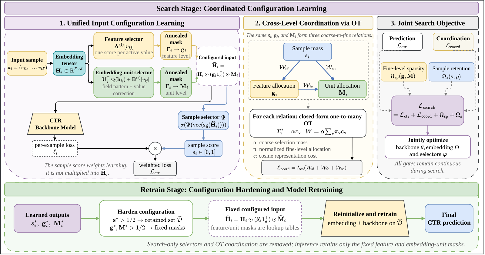
| Search | Three selectors are trained jointly with the CTR model, masks are continuous; total loss = weighted CTR loss + consistency penalty + sparsity constraints | A feature score and unit scores per feature value, a score per sample |
| Hardening | Every score becomes 0 or 1 at a 0.5 threshold | A retained sample set and two fixed mask tables |
| Retrain | Selectors and penalties are removed; training restarts from an intermediate search checkpoint on the retained samples | The final CTR model |
| Serving | New samples look up both mask tables by their feature values | The sample selector is not deployed, so it adds no cost |
The key design choice is the order of the selectors: the feature and unit selectors first decide what the model can see, then the sample selector judges whether a sample is worth learning from based on the processed input. That way the sample-level judgment rests on what the model actually receives.
How does each selector score?
The feature selector is the simplest: each feature value has a learnable score that passes through a sigmoid into a gate between 0 and 1, multiplied onto that feature's whole embedding. It answers whether a feature value takes part at all.
The unit selector answers a finer question: which dimensions of a kept feature are useful. Each feature field gives each of its 16 dimensions a learnable vector, shared by all values of that field; the current embedding is dotted with each of these 16 vectors and a per-value bias is added, giving a score for each dimension. The field-shared part learns patterns common to that type of feature, and the bias corrects for individual values.
Why add temperature annealing? Early in search the masks are smooth continuous values, so gradients reach many candidate configurations. As epochs pass, the coefficient inside the sigmoid grows, masks move closer to 0 or 1, and thresholding at the end of search loses less.
The sample selector is a small MLP that takes the tensor already multiplied by both masks and outputs the sample's weight. To stop it from deleting everything, one loss term keeps the average retention near 98%, and an entropy penalty pushes each weight toward 0 or 1.
The consistency penalty: what does the "optimal transport" in the title actually do?
When the three selectors are linked only through the prediction loss, an upper level has no idea where a lower level puts its weight. What the authors want is this: if a sample gets high weight, its feature gates should concentrate on features whose embeddings are close to the sample's overall representation; likewise, if a feature is kept, its unit mask should concentrate on dimensions close to it.
The paper writes each upper–lower pair as an optimal-transport problem: the upper level's weight is the total mass to ship, the lower level's normalized gates decide where it goes, and the cost is the cosine distance between their representations. Because there is only a single source, the transport problem has a closed-form solution, which is just a weighted average:
Here is the sample weight, the share derived from the feature gates (as with the unit masks below: log, divide by a temperature, then softmax over the sample's features), the mean of the sample's feature embeddings, and is one minus cosine similarity. All three penalties use the raw embeddings, before any mask, which the authors say gives a stable anchor while the masks are still changing; gradients from the penalties flow back into these embeddings and the unit vectors. A worked example (illustrative): sample weight 0.9, two features with normalized gates 0.8 and 0.2, whose cosine distances to the sample mean are 0.1 and 0.7. The penalty is 0.9×(0.8×0.1+0.2×0.7)=0.198. Flip the gates to 0.2 and 0.8 and the penalty rises to 0.9×(0.02+0.56)=0.522. So the term says: the larger a sample's weight, the more its gates must sit on features close to the sample as a whole. Hoot says

Gates favour the near feature
- Feature A: gate 0.8 × distance 0.1
- = 0.08
- Feature B: gate 0.2 × distance 0.7
- = 0.14
- × sample weight 0.9
- penalty 0.198
Most of the weight sits on the near feature: small penalty.
Gates swapped, favouring the far feature
- Feature A: gate 0.2 × distance 0.1
- = 0.02
- Feature B: gate 0.8 × distance 0.7
- = 0.56
- × sample weight 0.9
- penalty 0.522
Distances unchanged, gates moved: the penalty grows about 2.6 times.
Sample weight 0.9; feature A's cosine distance to the sample mean is 0.1 (near), feature B's is 0.7 (far). Illustrative numbers. Source: paper's consistency penalty W_sf(i) = s_i Σ_j π_ij c(h̄_i, h_ij), c = one minus cosine similarity; numbers are the article's illustrative example
The other two terms have the same form. Each embedding dimension has a learnable dimension vector, which is also what scores that dimension. The feature-to-dimension term, weighted by the feature gate, measures the cosine distance between the feature embedding and the vectors of the dimensions it keeps. The sample-to-dimension term skips the feature level. The unit masks of all fields in the sample are lined up, each value is logged and divided by a temperature, and one softmax over all of them gives shares that sum to 1. These shares weight the cosine distances between the sample's average representation and each unit vector, and the sum is multiplied by the sample weight. Put plainly, no transport plan is solved here; what works is a cosine-distance penalty weighted by the upper level and distributed by the lower level's gates. The form is sensible, but readers need not be intimidated by the name "optimal transport", nor should they expect extra properties from transport theory.
Results
Experiments use four public datasets: Avazu, Criteo, MovieLens-1M and Alibaba's AliCCP, all with 16-dimensional embeddings. Each method is attached to five backbones (DNN, DeepFM, DCN, AutoInt, FinalMLP), and results are means over five random seeds. The table below shows AUC with the DNN backbone:
| Method | Avazu | Criteo | MovieLens-1M | AliCCP |
|---|---|---|---|---|
| No selection | 0.7893 | 0.8097 | 0.8151 | 0.6243 |
| OptFS (feature selection) | 0.7907 | 0.8107 | — | 0.6245 |
| AutoDenoise (sample selection) | 0.7834 | 0.8104 | — | — |
| IDC (joint three levels, no penalty) | 0.7915 | 0.8110 | 0.8174 | 0.6256 |
| OptIDC | 0.7930 | 0.8113 | 0.8181 | 0.6263 |
OptIDC gets the highest AUC on all four datasets and all five backbones, and its gap over the strongest baseline is significant at p≤0.05. But look at the size: on Criteo it is only 0.0016 above no selection and only 0.0003 above IDC. Most of the gain comes from learning the three levels together; the consistency penalty contributes most visibly on Avazu and only adds a little elsewhere. Also, on AliCCP the DNN's LogLoss goes from 0.1616 to 0.1619: AUC improves while the overall accuracy of the predicted values slips slightly.
The ablation breaks the parts apart (Avazu, DNN backbone):
| Variant | AUC |
|---|---|
| Feature + unit selection, no penalty | 0.7910 |
| Feature + unit selection, with its penalty | 0.7920 |
| Joint three levels, no penalty (IDC) | 0.7915 |
| Without the sample-to-unit penalty | 0.7929 |
| Full OptIDC | 0.7930 |
| Three existing methods stacked (AOP) | 0.7912 |
Two points in this table stand out. First, doing only the feature and unit levels with the penalty between them already beats the three-level joint model without penalties; with the FinalMLP backbone this two-level version reaches 0.7938, almost the same as full OptIDC at 0.7941. That is not enough to say feature–unit alignment is the main source of the gain: dropping the sample level also drops the two sample-related penalties, so their effects cannot be separated. With DNN, adding the penalty to feature + unit selection gains 0.0010, and going on to full OptIDC with sample selection and the other two penalties gains another 0.0010. Second, stacking three existing methods gives only 0.7912, 0.0018 below OptIDC: "learning together" has to be designed along one information path, and simple stacking is not enough.
The authors also tried several simpler consistency constraints, and swapping cosine distance for Euclidean distance, and all perform about the same as IDC. What works is the specific combination of upper-level weight × lower-level allocation × cosine distance between representations, not just any consistency constraint.
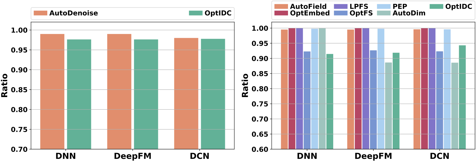
The retention ratios show that OptIDC's gain does not come from keeping more information: it drops about 2.4% of samples and 6% to 9% of embedding parameters and still gets higher AUC.
On cost, total training time on Avazu is 2575 seconds, about 2.4 times the 1069 seconds without selection, because it searches and then retrains; per-batch inference time rises from 0.0034 to 0.0041 seconds, from the mask-table lookups.
Limitations as I see them
First, the absolute gains are small, and one signal points the other way. On Criteo OptIDC is only 0.0003 AUC above IDC. AliCCP, the only one of the four datasets from a real e-commerce platform, sees LogLoss move from 0.1616 to 0.1619. For ads, where predicted values must be accurate, AUC and LogLoss moving in opposite directions needs to be understood first.
Second, it is far from industrial scale. Embeddings are only 16-dimensional, the largest dataset has about 38 million training samples, and there is no online experiment. The unit selector stores a 16-dimensional bias for every feature value, which amounts to another table as large as the embedding table; industrial models often have hundreds of millions of feature values, so memory and storage during search would multiply.
Third, the tuning burden is heavy. Feature sparsity, unit sparsity, sample retention, entropy penalty and consistency penalty each have a weight, plus the annealing coefficient and the retraining checkpoint, and the paper grid-searches every one. Averaged over five backbones, the consistency penalty's gain is on the order of a thousandth, so the tuning cost may well exceed the benefit.
How a recommendation team could try it
- First check whether existing feature selection and embedding compression "fight": count how many switched-off features still have unit masks being trained, and how many down-weighted samples have high feature gates. Joint learning only has room if conflicts are common.
- Start with just the feature and unit levels plus the paper's cosine-distance penalty. On some backbones this pair already comes close to full OptIDC (0.7938 vs 0.7941 on FinalMLP), so it is a reasonable starting point; sample selection most easily overlaps with existing denoising and sampling logic and can be added later.
- Watch LogLoss and calibration metrics as well as AUC. If overall prediction accuracy worsens, add calibration after retraining or lower the penalty weight.
- Estimate the mask-table cost: number of feature values times embedding dimension, and see whether it fits during search; if not, apply unit selection only to high-frequency fields.
Verdict
The three input-side trims can be learned together in one framework, and tuning them separately tends to cancel out. That view is worth taking away more than the specific method.
| Dimension | Assessment |
|---|---|
| Problem importance | Medium. Feature and embedding selection is a mature area; the joint view is new, but single-level gains are largely exhausted |
| Method novelty | Medium. Unifying everything as masks is clear; the "optimal transport" is really a weighted cosine penalty |
| Experimental evidence | Medium-low. Four public datasets, five backbones, five seeds, significant but small; LogLoss worsens on AliCCP; no online test |
| Engineering cost | Medium-high. About 2.4× training time, an extra bias table as large as the embedding table, many hyperparameters |
| Worth trying? | Borrow a simplified "joint feature-and-unit selection + consistency penalty"; do not adopt the full method as is |
How did this read for you?
Hoot made a note. Thanks for the feedback.

One tap, no sign-in; tap again to undo. Only anonymous counts are kept, never who you are.
Discussion
Add experiment details, reproduction notes or a different take. Requires a GitHub sign-in.
Loading the discussion…