Contents · 8 sections
1Three stages in a vector retrieval pipeline2Evaluated objects and evaluation conditions3Walking through it: who is to blame for a low recall on MSCOCO4The index is about speed and retention5Filtered search: bigger parameters, lower recall6Filter ratio and dimensionality decide whether to use an index7What this means for people running vector search8LimitationsSHARE

Vector search recall won't go up: swap the embedding, swap the index, or tune parameters? VecDBLens splits the billYour image-text search has been live for a while and its recall stays low. A user types a description of a picture, the system searches over a million images, and the paired image often fails to make the top 10. It is tempting to start by tuning the index: raise HNSW's efSearch, or replace IVFPQ (an inverted-file index with product-quantization compression) with HNSW (a hierarchical graph index).
One number in the paper is worth pausing on. On VisualNews, a news image-text dataset, encoded with SigLIP2 and searched exactly, without any index, over 1,259,732 candidate images, only 408 of 20,000 image descriptions have the paired image as their nearest image, which is 2.04%. No index is involved at that point; the problem lies elsewhere.
This paper, from the Institute of Computing Technology of the Chinese Academy of Sciences, the University of Chinese Academy of Sciences, The Chinese University of Hong Kong, Shenzhen, and Universiti Sains Malaysia, asks one question: when vector retrieval misses its recall and throughput targets, should you blame the embedding, the index, or the way queries are searched? Most existing vector database benchmarks fix one embedding and compare only indexes; they also often use exact nearest neighbors as ground truth, which may not match real relevance, so embedding problems get charged to the index. Their configuration ranges are narrow too, which favors systems that happen to suit a particular configuration. VecDBLens treats one stage at a time as the evaluated object, fixes everything else (dataset, workload, parameters, hardware) as one shared set of conditions, compares only under identical conditions, and then uses variance analysis to see how the stages affect each other. The paper runs one diagnosis on image-text retrieval and one on filtered vector search.
Exact-search recall under a given embedding is the reference line for diagnosis; in the image-text experiments graph indexes keep about 99% of it and the bottleneck is mostly the embedding. In filtered search, though, tuning index parameters more aggressively can lower recall. These findings come from offline measurements on public datasets.
Three stages in a vector retrieval pipeline
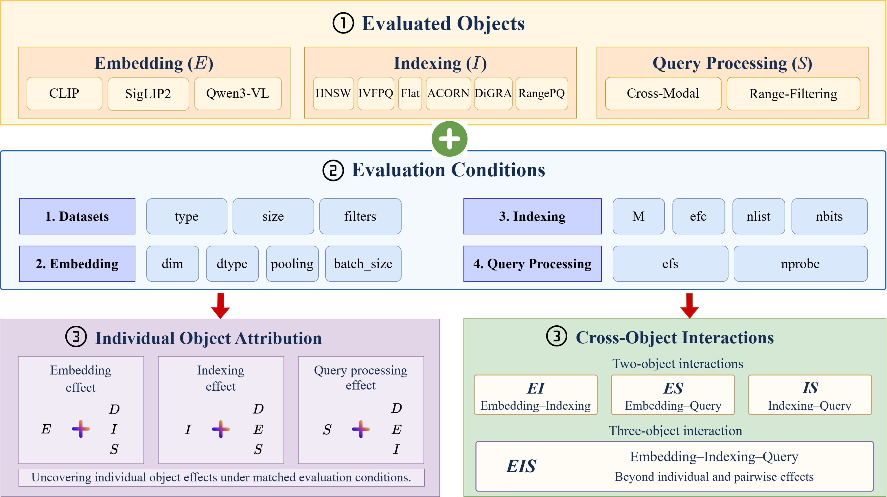
The paper splits vector retrieval into three steps. The first is the embedding: encoding raw objects such as images and text into vectors. The second is indexing: organizing the vectors with algorithms like HNSW, IVFPQ or CAGRA (a graph index that runs on GPUs), each with its own build parameters, such as how many edges each HNSW node gets. The third is query processing: searching the index, again with parameters, such as how many candidates HNSW explores per search (efSearch) or how many buckets IVFPQ probes (nprobe).
Low recall can come from any of the three. The embedding may place related images and text far apart; the index may fail to keep the neighbor relations the embedding defines; the search method may become inefficient once filters are added. From the final recall number alone you cannot tell which step it is.
There is also a reference: Flat, exact search that builds no index and computes every distance. For a fixed embedding, Flat gives the most accurate distance ranking available in that vector space. The paper uses it as the reference line: an index only decides how fast you search and how much of it you keep, and cannot change which images and texts the embedding puts close together.
Evaluated objects and evaluation conditions
VecDBLens borrows the vocabulary of Evaluatology: each diagnosis answers one question, the stage being compared in that question is the evaluated object, and every other factor is an evaluation condition.
The same factor plays different roles in different questions. When comparing embeddings, the embedding is the evaluated object and the dataset, index configuration, search parameters and hardware are conditions; when comparing indexes, the embedding becomes one of the conditions. Comparisons are made only under shared conditions: to compare two indexes such as ACORN (a graph index that supports filters) and RangePQ (a compressed index organized by attribute range), you use the same vectors, the same queries, the same search settings and the same hardware.
After comparing single objects, the next question is how they interact. The paper uses functional analysis of variance (ANOVA) to split the variation in recall retention and throughput into parts: the average effect of the embedding, of index construction and of query processing on their own, plus the extra effect that appears when two or all three act together. The latter are called interaction terms.
Walking through it: who is to blame for a low recall on MSCOCO
Below we use the MSCOCO (a common image-text retrieval dataset) full candidate pool numbers from the paper's Table 1, Table 13 and Fig. 2, following the diagnosis in order.
Step 1, spot the problem. With SigLIP2 embeddings and an HNSW index, the Fig. 2 label for this cell shows Recall@10 of about 0.047, meaning fewer than 5 in 100 descriptions find their paired image in the top 10. It looks as if the index was built badly.
Step 2, fix the embedding and switch to Flat. The evaluated object is the index; the conditions are SigLIP2 and this dataset. Flat's Recall@10 is 0.0488. Retention = 0.047 ÷ 0.0488 ≈ 0.96, which shows the index loses only about 4%.
Step 3, fix Flat and swap the embedding. Now the evaluated object is the embedding; the conditions are Flat and this dataset. CLIP's Flat recall is 0.2973 and Qwen3-VL's is 0.5998. Going from SigLIP2 to Qwen3-VL raises the reference line from 0.0488 to 0.5998, more than 12 times higher, which shows the bottleneck is the embedding.
Step 4, count the cost. Qwen3-VL vectors have 4096 dimensions, CLIP vectors 512. On this candidate pool, CLIP's Flat runs 207.18 queries per second and Qwen3-VL's only 24.94, 8.31 times slower. Swapping the embedding buys recall and gives up throughput.
Step 5, bring the index back. The evaluated object is the index again, now under Qwen3-VL. Graph indexes keep a high average share of exact-search recall: 0.9959 for CAGRA and 0.9875 for HNSW. In Fig. 2, Qwen3-VL with HNSW on this pool is labelled 0.599, almost the same as Flat's 0.5998, so the index can win back throughput.
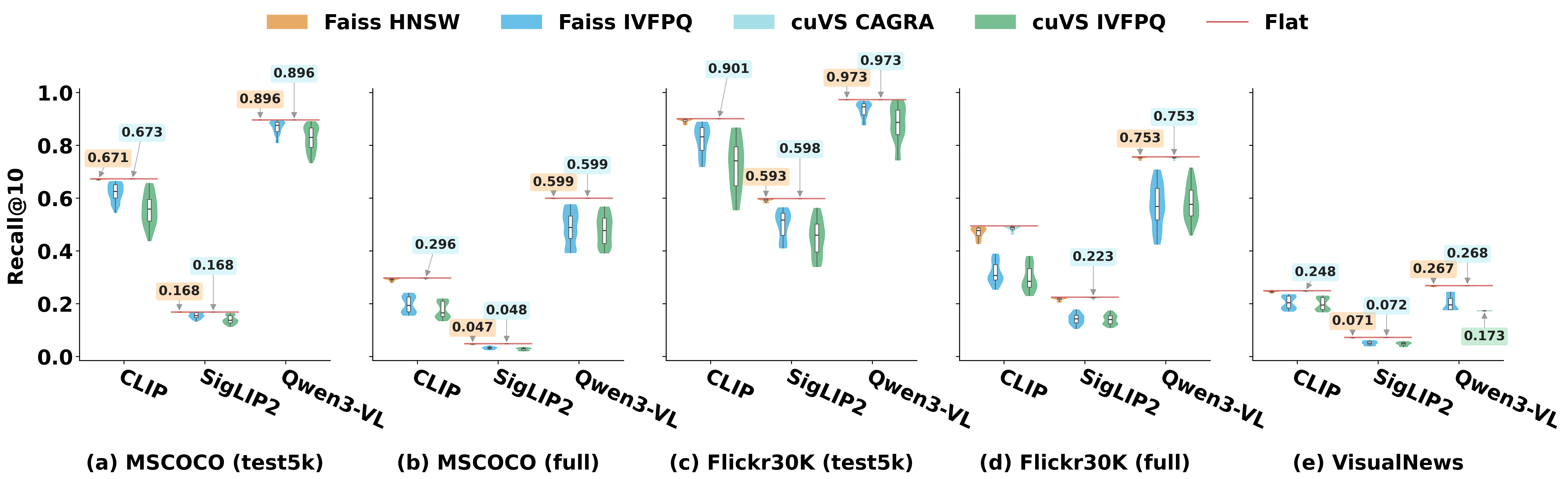
This example shows that measuring the reference line with Flat first, when recall is low, tells you whether the index is losing results or the embedding never put the related images and texts together. The paper lists Flat recall for five conditions in one table:
| embedding | dimensions | MSCOCO full pool | VisualNews | mean of five conditions |
|---|---|---|---|---|
| Qwen3-VL | 4096 | 0.5998 | 0.2687 | 0.6988 |
| CLIP | 512 | 0.2973 | 0.2496 | 0.5230 |
| SigLIP2 | 768 | 0.0488 | 0.0724 | 0.2225 |
(Numbers from the paper's Table 1 and Appendix B.2, Flat exact-search Recall@10. The five conditions are the 5,000-image test pool and the full pool of Flickr30K and of MSCOCO, plus VisualNews.)
These differences are not just a matter of dimensionality. When the paper reduces SigLIP2 and Qwen3-VL to the same 512 dimensions as CLIP, the pairwise differences among the three models remain statistically significant.
Good embeddings also hold up better as the candidate pool grows: going from 5,000 images to the full pool, Qwen3-VL keeps 72.3% of its recall, CLIP 49.6%, and SigLIP2 33.2%.
The index is about speed and retention
Since the embedding sets the reference line, the index's job is to keep it with as little computation as possible. With CLIP on VisualNews, Flat runs only 13.81 queries per second, so an index is needed for speed. Among configurations with retention of at least 0.99, HNSW reaches 1,898.56 queries per second on 28 CPU threads, and CAGRA reaches 29,433.58 on one V100 with 99.28% retention. This compares whole backend-plus-hardware setups, one on CPU and one on GPU, so the throughput ratio cannot all be credited to the index algorithm.
Compressed indexes pay in recall. Faiss IVFPQ's mean retention is 0.7932 and cuVS IVFPQ's is 0.7409; they trade recall for memory.
For HNSW, interactions among the three stages show up mainly in recall and hardly at all in throughput: interaction terms explain 19.34%–22.01% of the variation in recall retention but only 0.67%–1.75% of throughput. One concrete sign is that raising efSearch 8 times shrinks the standard deviation of retention across index build configurations by 36.0%–78.0%, which means that searching a bit more at query time makes the choice of build parameters matter less.
Filtered search: bigger parameters, lower recall
The second set of experiments is filtered vector search, such as "find the most similar items within a given price range". The data are 990,000 vectors derived from SIFT1M (a classic million-scale image-feature vector benchmark) and GIST1M (a similar high-dimensional benchmark), with 128 and 960 dimensions, plus scalar attributes for range filtering, at filter ratios from 0.01% to 50%.
The paper runs a monotonicity audit: under identical conditions, raise one index build parameter by one level and record whether recall drops. Raising ACORN's per-node edge count M drops recall in 273 of 2,244 comparisons, 12.2%, with a largest drop of 0.4332, so raising a parameter is not always safe; raising efConstruction, the search width used while building the graph, drops it in 18.2% of cases, with a largest drop of 0.5237. Raising DiGRA's M drops recall in 25.6% of cases, but by small amounts.
One ACORN comparison makes it concrete:
| Metric | Original graph | Graph with more edges |
|---|---|---|
| Average filter-compatible neighbors per node | 0.1596 | 0.2002 |
| Share of nodes eligible for two-hop expansion | 59.97% | 18.78% |
| Recall@100 | 0.3150 | 0.1827 |
(Numbers from the paper's Table 4.)
With more edges, each node does have slightly more usable neighbors on average; but when the graph has more edges, ACORN also raises the threshold for "looking at neighbors of neighbors", so the share of nodes eligible for two-hop expansion falls from six in ten to under two in ten, and recall falls from 0.3150 to 0.1827. The paper gives a second reason: with a wider search during construction, the graph gets longer edges pointing in less varied directions, so a query visits more nodes yet reaches fewer true neighbors. On two real workloads, CC-News and App Reviews, raising efConstruction from 100 to 400 lowers recall in 39 and 35 of 78 comparisons respectively.
Filter ratio and dimensionality decide whether to use an index
With filters, filtering first and then searching exactly (Flat pre-filtering) is not always slow. On 128-dimensional SIFT at a filter ratio of only 0.01%, Flat runs 8,949.74 queries per second and is the fastest, because few vectors pass the filter and need a distance computed. At 10%, Flat drops to 48.07 queries per second while single-threaded DiGRA reaches 1,592.11.
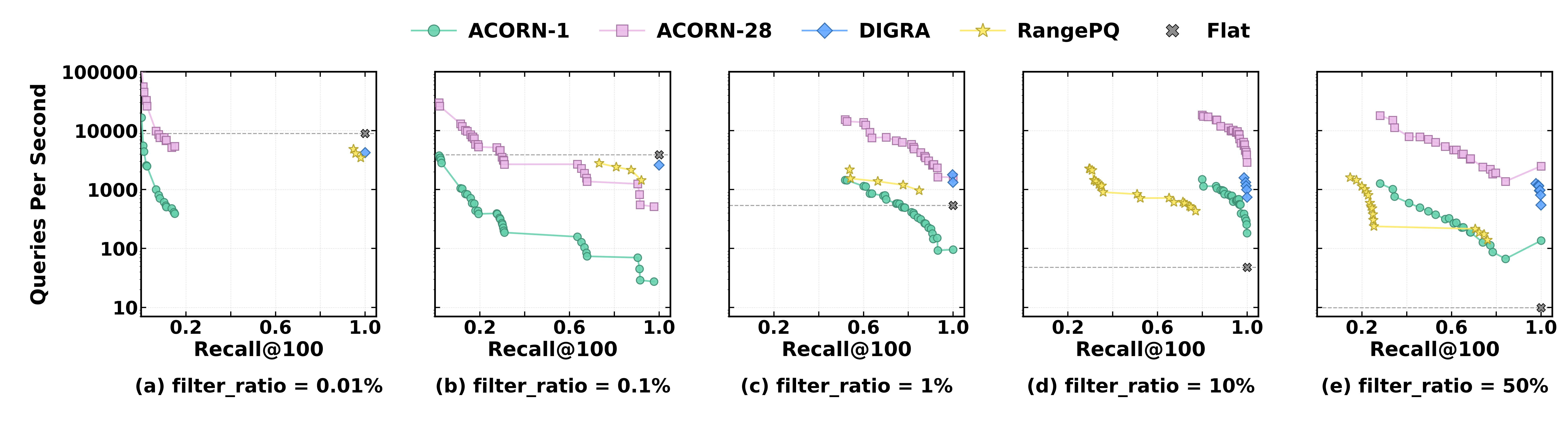
On 960-dimensional GIST, each distance computation costs more, and among tested configurations that reach Recall@100 of 0.95, DiGRA is the fastest single-threaded method at every filter ratio, including 0.01%: 3,843.01 queries per second against Flat's 1,158.62. So under the tested 960-dimensional conditions, Flat is not the fastest even with the strictest filter.
Beyond speed there is the cost of building the index. At 128 dimensions, DiGRA's median build time is 6,162 seconds, while single-threaded ACORN needs only 3.71 seconds. RangePQ builds fast and adds the least memory, but on 960-dimensional GIST none of its tested configurations reaches Recall@100 of 0.95.
What this means for people running vector search
When recall misses the target, first measure the reference line with Flat on the same vectors, then decide whether to work on the embedding or the index first.
If Flat itself is low, check the embedding first, and use retention to see how much room the index and search parameters still have; after moving to a larger embedding, use a graph index to win back throughput. If Flat is high and the index is low, the problem is the index and query parameters, and a good first step is a larger search budget at query time, which reduces sensitivity to build parameters.
When tuning build parameters for filtered search, do not assume bigger is better. At your own filter ratio and dimensionality, run two adjacent parameter levels under identical conditions and check whether recall actually drops. Whether to use Flat pre-filtering also depends on filter ratio and dimensionality together.
Limitations
VecDBLens looks at recall, throughput, memory, build time and parameter stability. It can point to the stage where the bottleneck lies, but cannot say which kinds of semantics the embedding gets wrong. The paper lists finer semantic diagnosis as future work.
Image-text retrieval uses Flickr30K, MSCOCO and VisualNews; the main filtered-search experiments use SIFT and GIST with synthetic scalar attributes, and the real workloads were added only for ACORN. Throughput numbers depend on the paper's hardware, two Xeon Gold 6330 CPUs and V100 GPUs; on other hardware the exact ratios will change.
How did this read for you?
Hoot made a note. Thanks for the feedback.

One tap, no sign-in; tap again to undo. Only anonymous counts are kept, never who you are.
Discussion
Add experiment details, reproduction notes or a different take. Requires a GitHub sign-in.
Loading the discussion…