Contents · 7 sections
1Six steps from one query to one group of training examples2Settle the answer first, then write the query3Negatives: filter out false negatives, then pick three tiers4Training sets a minimum score gap for every pair of documents5Why not regress the teacher's gap directly?6A lower-bound constraint scores 1.23 points above yes/no alone7The 4B student beats the 8B teacher only with model mergingSHARE

When a reranker is trained only on "relevant" and "not relevant" labels, it struggles to rank irrelevant documents against each other. Tencent Yuanbao Search's Yuanbao-Reranker fills this gap by having a stronger teacher model score the documents and then requiring that, of any two documents, the one the teacher finds more relevant must get a student score higher by at least some margin, with no penalty for exceeding it.
In this paper's evaluation, an embedding retriever first fetches a batch of candidates from the corpus (100 per query), and then a reranker encodes the query together with each candidate, scores the candidates one by one, and reorders them. This paper comes from Tencent Yuanbao Search; the authors trained rerankers at three sizes, 0.6B, 4B and 8B, on top of Qwen3, collectively called Yuanbao-Reranker. The whole article uses one illustrative query: "Must a company pay severance if it dismisses an employee for failing to meet hiring requirements during probation?" In the illustration, document A answers the question directly, B covers the conditions for ending a contract during probation, C covers how severance is calculated, and D covers the minimum wage during probation.
The difficulty is that B, C and D, like A, all talk about probation, dismissal and compensation, so a reranker looking only at keywords can hardly tell the four apart. What a reranker must check is whether a document meets the specific conditions in the query: here the conditions are "during probation, on the ground of not meeting hiring requirements" and the wanted answer is "pay or not pay", and only A meets both. Training such a model needs many "same topic, but does not answer" examples, while publicly labeled data covers a narrow range of domains and phrasings.
A typical reranker training pipeline has these parts. An LLM reads a document and writes a query for it to expand the data. The other documents a retriever returns for that query become negatives (examples of irrelevant documents). Each document is labeled yes (relevant) or no (not relevant), and supervised fine-tuning (SFT) teaches the model to output yes or no after reading the query and a document. The paper points out a problem in each part, and the first is in the data. The LLM may drop a condition and write "Does a company have to pay severance when dismissing an employee?", which a document about ordinary dismissal with no mention of probation can also answer, so the trained model never learns to check the "probation" condition. The LLM may also write the answer into the question, as in "Why is no severance owed when someone is dismissed for failing probation requirements?", so the model can find A by surface overlap alone and never learns to judge whether a document gives the answer. The retrieved results may also contain relevant documents nobody labeled, for example another legal Q&A, E, that also answers the question but is penalized as a negative; such a document is called a false negative.
The labels themselves are not enough either. With B, C and D all labeled no, SFT only tells the model that all three are irrelevant, not that B is closer to the question than D: B is precisely about ending a contract during probation, while D merely mentions probation too. The nearest existing remedy is to use an off-the-shelf strong reranker as a teacher and require the model being trained (the student) to give two documents a score gap as close as possible to the teacher's gap for them; this is called regressing the teacher's score gap. But if the student has already separated A and D further than the teacher did, the regression target pulls their gap back in.
This paper changes both the data and the training objective. On the data side, the authors have the LLM settle the answer from the document before writing the query, use teacher scores to filter out suspected false negatives, and give each query three negatives of different difficulty. On the training side, the authors keep the yes/no labels and add one constraint: of any two documents, the one the teacher scores higher must also be scored higher by the student by at least some margin, with no penalty for exceeding it. This constraint applies not only between A and the negatives but also among B, C and D. The final 4B model reaches an average nDCG@10 (a measure of how well the top 10 are ordered, reported on a 100-point scale) of 73.63 across five retrieval benchmarks covering Chinese, multilingual, English, long-document and code retrieval, above the 72.68 of its teacher, Qwen3-Reranker-8B.
Six steps from one query to one group of training examples
The table below shows the whole pipeline. The first five steps all happen during training. Only the single model merged in step 5 is deployed; it scores each candidate on its own and is used just like an ordinary reranker.
| Step | Input | Operation | Output | Training only |
|---|---|---|---|---|
| 1. Synthesize | Unlabeled documents | Settle the answer and its source evidence first, then write the query | Query and positive document | Yes |
| 2. Filter | Synthesized pairs | Teacher verification, query deduplication, quotas by source and length | Retained pairs | Yes |
| 3. Mine negatives | Retrieved candidates from a real corpus | Exclude suspected false negatives, take three by difficulty | A group of 1 positive and 3 negatives | Yes |
| 4. Train | A group and its teacher scores | yes/no cross-entropy plus pairwise minimum-margin constraints | Models at three sizes | Yes |
| 5. Merge | Several same-size models trained on different data mixes | Merge parameters layer by layer with weights | One model | Yes |
| 6. Serve | A query and one candidate | Compute the yes logit minus the no logit | This document's score | No |
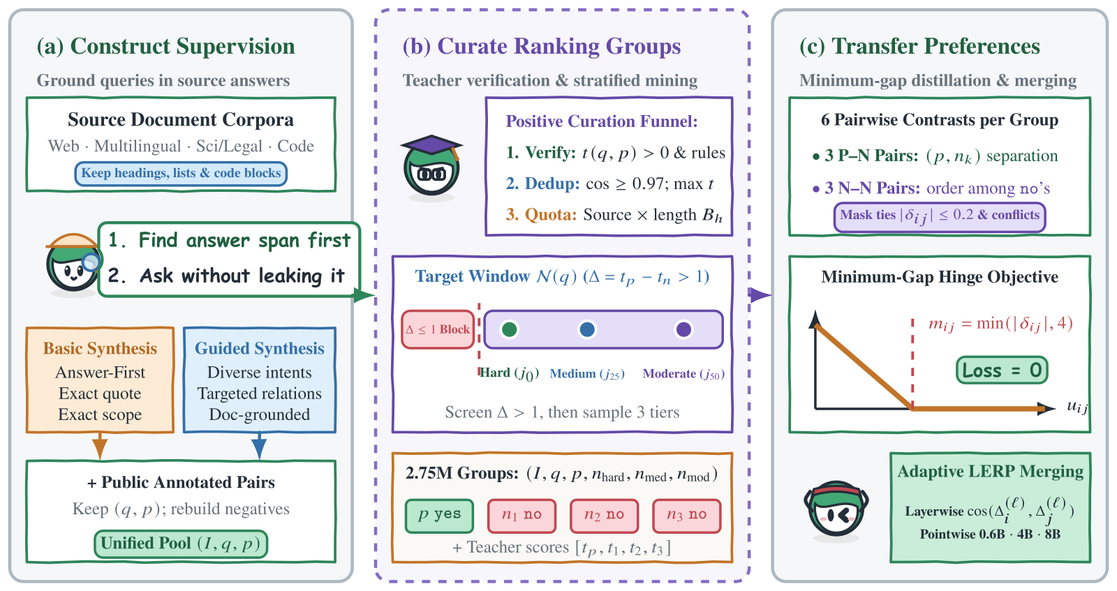
The teacher is the off-the-shelf Qwen3-Reranker-8B, and a teacher score is its yes logit minus its no logit, with a higher score meaning a more relevant document. After the first three steps, the probation query becomes the group below (illustrative), and every later mechanism works on it.
| Document | Content | Label | Teacher score | Negative tier |
|---|---|---|---|---|
| A | Directly answers whether severance is owed for dismissal during probation | yes | +5 | positive |
| B | Conditions for ending a contract during probation | no | +2 | Hard |
| C | How severance is calculated | no | −1 | Medium |
| D | Minimum wage during probation | no | −4 | Moderate |
Settle the answer first, then write the query
The usual approach has the LLM write a query right after reading a document. But sharing keywords with a query does not mean the document can answer it. So the authors reverse the order: the LLM reads the whole document, first settles a complete answer, then copies out verbatim the source text supporting that answer, and only then writes the query. The query must keep conditions such as entities, time and jurisdiction, and the answer stays in the document. After this step, the output for probation document A looks roughly like this (illustrative, some fields omitted):
{
  "status": "AUTHORED",
  "query": "Must a company pay severance if it dismisses an employee for failing to meet hiring requirements during probation?",
  "answer_proposition": "If the contract is ended because the employee failed to meet hiring requirements during probation, the company does not have to pay severance",
  "supporting_passages": [
    {"unit_id": "E1", "supporting_quote": "(a passage copied verbatim from document A)"}
  ],
  "no_answer_leakage_check": true
}
status is the outcome for this example, and AUTHORED means a query was successfully written; no_answer_leakage_check records whether the query passed the "does not leak the answer" check. This step has two independent checks. One requires the answer to be fully supported by this document, with the same scope as the query; the other requires every quoted passage to be found verbatim in the document, exactly once. The verbatim match only proves the quote really comes from the source; whether the answer fits the query rests on the first check, and teacher scoring later adds another gate. Documents from which no source text can be quoted are marked SKIPPED and dropped. A second synthesis route first picks a type of information need, such as troubleshooting software or finding the applicable regulation, then writes queries by type, following the same rules: settle the answer, quote the source, and keep the answer out of the query.
The authors synthesize only positives; all negatives come from a real corpus. In preliminary experiments, neither synthesized negative documents nor synthesized negative queries improved ranking. The authors' reasoning is that a synthesized negative document is too easy if it is far from the query and may actually answer it if it is close, and that LLM-written text carries stylistic traces, so the reranker being trained can spot negatives by style without reading the content.
Synthesized query-positive pairs then pass three filters. The first is verification: the teacher's score for the query and its positive must be above 0, meaning the teacher finds yes more likely than no, and pairs whose document only partly answers and scores too low are dropped. The second is deduplication: two same-language queries whose vectors have cosine similarity of at least 0.97 count as duplicates, mutually duplicate queries form a cluster, and only the query with the highest teacher score in each cluster is kept. The third is quota allocation, which handles bias by document length and source: short encyclopedia passages generally get higher teacher scores than long technical documents, so taking the global top scores would over-select short, easy sources.
Illustration: in one domain and language there are 100 candidates, 50 short, 30 medium and 20 long documents, and a budget of 10 slots. Taking the global top 10 might yield 10 short documents. Allocating slots in proportion gives 5, 3 and 2, so long documents are guaranteed 2 slots, and within each tier the highest teacher scores are taken. This shows that teacher scores only rank documents within one tier, while the proportions across tiers are set by the quotas.
The contribution of the synthetic data is measured this way: using the 0.6B version before model merging, the authors compare training on public labels only with training that adds synthetic data, with the same negative selection and training objective on both sides. The score is written Avg., the equal-weight average of nDCG@10 over five benchmarks (called panels below), which test Chinese (CMTEB-R), multilingual (MMTEB-R), English (BEIR), long-document (MLDR) and code (MTEB-Code) retrieval.
Avg. rises from 68.77 to 70.43, a gain of 1.66. MLDR rises 3.82 and MMTEB-R 2.37, while CMTEB-R and BEIR each rise only about 0.4. This shows the synthetic data mainly fills the long-document and multilingual cases that public labels lack, and adds little on the Chinese and English panels that public labels already cover well.
Negatives: filter out false negatives, then pick three tiers
Now look at how B, C and D are chosen. For each query the authors use a retriever to fetch candidates from a real corpus, have the teacher score each one, and compute Δ, the gap between the positive's teacher score and this candidate's. Candidates with Δ of at most 1 are treated as suspected false negatives and excluded outright. Illustration: A's teacher score is +5 and E's is +4.5, so Δ is only 0.5 and E is excluded, and the model is never penalized for scoring E high. B's Δ is 3, so B stays.
After filtering, the authors sort candidates by Δ from small to large and take three: the first, the one at the quarter mark and the one at the median, called Hard, Medium and Moderate; the easier half beyond the median is discarded. Illustration: 9 candidates remain after filtering, numbered 0 to 8; numbers 0, 2 and 4 are taken, and 5 through 8 are skipped. Hoot says

Candidates A–K and their Δ values are illustrative; the sampling rules are from the paper.
Source
paper §2.4 and Appendix A.4: each query stores a top-1,024 dense retrieval pool; known positives and near-duplicates are excluded and only candidates with Δ>1 are kept (Δ=t(q,p)−t(q,n)); sorted by ascending Δ, j0=0, j25=max(1,⌊0.25(m−1)+0.5⌋), j50=min(m−1,max(j25+1,⌊0.50(m−1)+0.5⌋)), m≥3; A–K and their Δ values are illustrativeWhy not simply take the three hardest? Three documents all from the hardest end would have teacher scores very close to each other. Illustration: if their Δ values are 1.2, 1.3 and 1.5, the pairwise teacher gaps are only 0.1 to 0.3, and there is almost no ordering among them to teach.
The effect of this step is also measured on the 0.6B unmerged version: with 1 random negative per query Avg. is 67.11, with 3 random negatives it is 68.44, and with 3 filtered and tiered real candidates it is 70.43, which is also the score of the full data setup on the 0.6B unmerged version. Going from 1 to 3 negatives adds 1.33 points, and replacing random negatives with filtered, tiered ones adds another 1.99. This shows that in this comparison, which negatives are chosen matters more than how many are used.
Training sets a minimum score gap for every pair of documents
The reranker's input is a task instruction (telling the model to judge whether this document meets the query), the query and one document, and after reading them the model predicts yes or no at the position where the answer goes. A document's score is the yes logit minus the no logit; for example, with a yes logit of 3 and a no logit of 5 (illustrative), the score is −2. At serving time each candidate is scored on its own, and higher scores rank higher.
A group of 4 documents gives SFT 4 yes/no judgments, and pairing them gives 6 pairs: the 3 pairs of A with B, C and D, and the 3 pairs among B, C and D. The authors add a hinge penalty with only a lower bound to every pair so that the student learns the teacher's ordering; this kind of learning from a teacher is called distillation:
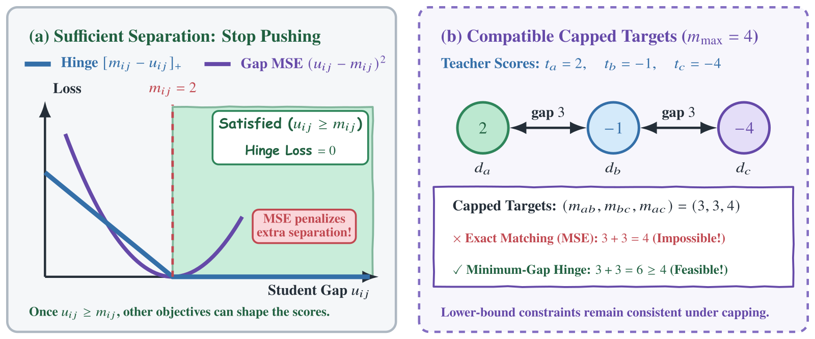
is the teacher score and the student score. is the minimum gap required for this pair, equal to the teacher's gap but capped at 4. is the student's gap measured in the teacher's direction, and it is negative if the student has the pair in the wrong order. means becomes 0 when it is below 0, so once the student's gap reaches the requirement , the penalty is 0 and widening the gap further costs nothing. This penalty is added to the SFT loss with weight 0.1. It makes documents in the same group compare scores only during training; at serving time each document is still scored on its own.
Illustration: a student trained with SFT alone gives A, B, C and D scores of +5, −2, −2.5 and −3. A is already well separated from the three negatives, but the three negatives are squeezed within 1 point of each other. Plugging into the formula:
| Pair | Teacher gap | Minimum requirement | Student gap | Hinge penalty | Squared error (for comparison) |
|---|---|---|---|---|---|
| A and B | 3 | 3 | 7 | 0 | 16 |
| B and C | 3 | 3 | 0.5 | 2.5 | 6.25 |
| B and D | 6 | 4 | 1 | 3 | 9 |
Both hinge penalties fall among B, C and D, exactly where yes/no labels have no say. The gap between A and B already exceeds the requirement, so this pair's penalty is 0 and SFT is free to keep adjusting both scores.
Why not regress the teacher's gap directly?
Look at the last column of the table. If the minimum requirement became an exact target regressed with squared error, the largest penalty, 16, would land on A and B, a pair that is already well separated. That penalty pushes A's score down and B's score up, while SFT is pushing A toward yes and B toward no, so the two objectives cancel each other.
The cap of 4 spares the student from copying the teacher's very large gaps: the teacher's gap between A and D is 9, but the student only needs a gap of 4. The cap also creates a problem. The teacher scores of B, C and D, +2, −1 and −4 (the same numbers as the paper's Figure 4), give three targets of 3, 3 and 4. If B is 3 above C and C is 3 above D, then B must be 6 above D and cannot also be exactly 4 above it, so no three scores can bring the squared error to 0.
A lower bound has no such conflict: B being 6 above D satisfies "at least 4 above". And the teacher's own scores always satisfy every lower bound, because each pair's teacher gap is no smaller than its capped requirement, so these constraints always have a solution.
Two more cases are left out of this constraint. Pairs whose teacher gap is at most 0.2 are skipped; for example, if C and D had teacher scores of −1.0 and −1.1, the pair would not be compared, because the teacher gives almost no ordering. When the teacher ranks some negative above the positive, its preference conflicts with the positive label, and the paper trusts the label, so the whole group skips distillation and trains only on its yes/no labels.
A lower-bound constraint scores 1.23 points above yes/no alone
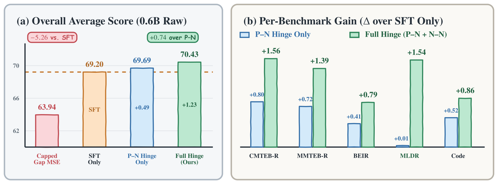
On the 0.6B unmerged version, the authors compared four training objectives with the same initialization, data and number of training steps, changing only the loss.
| Training objective | What is added to yes/no | Avg. | Relative to SFT Only |
|---|---|---|---|
| SFT Only | nothing | 69.20 | — |
| Capped Gap MSE | Regress the capped teacher gap on eligible pairs | 63.94 | −5.26 |
| P–N Hinge | Lower-bound constraints on the 3 positive-negative pairs only | 69.69 | +0.49 |
| Full Hinge (this paper) | Lower-bound constraints on all 6 pairs | 70.43 | +1.23 |
The same teacher gaps score 5.26 points below yes/no alone when used as a regression target, and 1.23 points above yes/no alone when used as a lower bound.
The authors explain the drop of Capped Gap MSE (mean-squared-error regression on the capped teacher gaps) with exactly the two things computed in the previous section: pairs that are already separated get pulled back, and the capped targets contradict each other. Full Hinge's 0.74-point lead over P–N Hinge is 60% of the total gain from distillation. This shows that most of the gain from distillation comes from the 3 pairs among B, C and D, and the 3 positive-negative pairs contribute less. Adding the pairs among negatives raises the long-document panel MLDR from 66.80 to 68.34.
Where the two models differ in ordering negatives shows up on 1,000 groups the authors held out from training. Each group has 1 positive and 3 negatives, with the negatives split into Hard, Medium and Moderate tiers as in training.
| Metric | SFT Only | Full Hinge |
|---|---|---|
| Pairwise accuracy of positive ranked above negative | 99.7% | 99.7% |
| Hard ranked above Medium | 71.6% | 90.5% |
| Medium ranked above Moderate | 58.7% | 78.1% |
| All three tiers in the right order | 36.4% | 69.7% |
| Average score gap between Hard and Moderate | 1.95 | 6.29 |
The first row is identical, which shows yes/no is already enough to put A ahead of B, C and D. The whole difference is in the last four rows: with yes/no alone, the average spread across the three negative tiers is only 1.95, and only 36.4% of groups have all three tiers in the right order; Full Hinge widens the spread to 6.29 and raises the fully ordered groups to 69.7%. The tier order itself is set by teacher scores, so this table measures how much of the teacher's ordering of negatives the student has learned. The same Full Hinge model scores 1.23 points of Avg. above SFT Only across the five panels, so in this comparison better ordering of negatives and a higher total score show up together.
The 4B student beats the 8B teacher only with model merging
First, the merge step from the pipeline table. Starting from the same Qwen3 checkpoint, the authors train one main model and several auxiliary models with different data mixes and training configurations, then merge parameters layer by layer with Adaptive LERP (linear interpolation whose weights are adjusted per layer). For each layer, they first compute each auxiliary model's direction of parameter change relative to the main model (the auxiliary model's parameters in this layer minus the main model's), and the more the auxiliary models agree in direction, the more weight they get in this layer. If the whole model used one fixed ratio, layers where the directions disagree strongly would also mix in the auxiliary models' parameters at that same ratio.
Illustration: there are 2 auxiliary models. In one layer their directions agree completely, with cosine 1, so each auxiliary model gets 0.25 and the main model 0.5. In another layer their directions disagree, with cosine no greater than 0, so each auxiliary model gets only 0.0625 and the main model 0.875. So the main model keeps at least half the weight in every layer, the merged result deployed is still one model, and inference cost is unchanged.
The main experiment has every reranker rerank the same top-100 candidates fetched by Qwen3-Embedding-0.6B, so first-stage recall is identical.
| Size | Qwen3-Reranker, same size | Yuanbao before merging | Yuanbao after merging | Lead over Qwen3 after merging |
|---|---|---|---|---|
| 0.6B | 67.32 | 70.43 | 70.96 | +3.64 |
| 4B | 72.13 | 72.64 | 73.63 | +1.50 |
| 8B | 72.68 | 73.34 | 74.21 | +1.53 |
This table answers which model is stronger at the same size: Yuanbao-Reranker beats Qwen3-Reranker of the same size at all three sizes, and the 8B version is the best on all five panels. The 0.6B model's 70.96 is also above every 1B–4B baseline outside the Qwen3 family, for example KaLM-Reranker-Large-R2 at 69.73.
The 4B model beating its teacher needs a closer look. The teacher is the 8B Qwen3-Reranker in the table, at 72.68. The 4B model is at 72.64 before merging, 0.04 below the teacher, and reaches 73.63 only after merging. So on this candidate pool, the 4B model beats the teacher only once merging is counted.
The authors' explanation is that the synthetic data widens the coverage of verified positives, and the hinge only demands local lower bounds, so the student does not have to imitate the teacher's mistakes when it scores documents one by one. The earlier ablations were all on 0.6B, so applying this explanation to 4B and 8B is the authors' inference.
With a different first-stage retriever, the conclusion keeps its direction. Switching to the top-100 fetched by Harrier-OSS-v1-0.6B, the three sizes' Avg. beats same-size Qwen3-Reranker by 4.03, 2.55 and 2.37, and the 4B model's 74.37 is also above the teacher's 72.30. This shows that although the lead changes with the candidate pool, it does not depend on the one retriever used in the main experiment.
Back to the probation query. At serving time the model still gives A, B, C and D one score each; the inference interface and model architecture are unchanged. The gains come from three places: data construction (answer-first synthesis, teacher screening, tiered negatives), up to six "at least this far apart" requirements per group during training (up to three of which govern the order of B, C and D), and parameter merging after training. What I take away is this recipe: when you have a strong reranker, using its score gaps, capped, as lower bounds is safer than using them as regression targets; in the same 0.6B experiment the former gains 1.23 points and the latter loses 5.26.
How did this read for you?
Hoot made a note. Thanks for the feedback.

One tap, no sign-in; tap again to undo. Only anonymous counts are kept, never who you are.
Discussion
Add experiment details, reproduction notes or a different take. Requires a GitHub sign-in.
Loading the discussion…